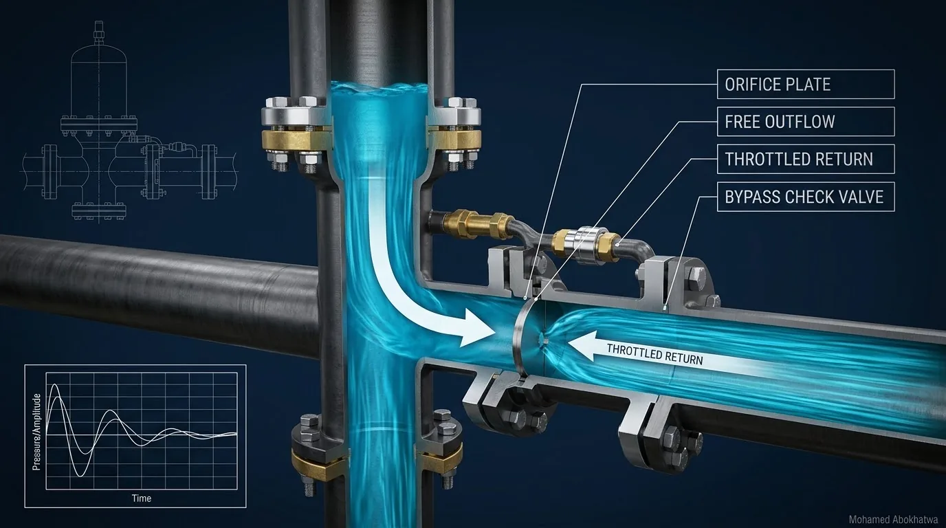
A surge vessel is specified by its gas volume, but whether that gas protects the pipeline is decided by the short pipe joining the vessel to the main. On the downsurge the vessel must discharge with as little loss as possible, because every bit of flow the connection holds back leaves as downsurge in the line. On the return, the water flowing back into the vessel carries the energy that becomes the upsurge, so that is the direction to throttle. On a 12 km DN800 main with a 20 m³ vessel holding 3.5 m³ of gas, a differential connection (outflow K 2, inflow K 10) in place of a free one cuts the maximum from 127.5 m to 119.2 m while the minimum moves only from +4.5 m to +4.3 m. A symmetric K 25 orifice, a plate of about 210 mm both ways, drops the line to −4.5 m.
1 · The connection is part of the vessel
Vessel data sheets list volumes and pressures; the connection appears as a nozzle size. Hydraulically that is backwards. The gas volume sets how much water the vessel can give. The connection decides how fast it gives it and how fast it takes it back, and those two rates set the two ends of the transient envelope.
The reference system
Every number here comes from one pipeline: a 12 km DN800 ductile iron K9 main [1], laid flat, carrying 2,520 m³/h (0.70 m³/s, 1.39 m/s) at a wave speed of 1,050 m/s, with the grade line at 85.0 m at the pump and 44.8 m at delivery. The pipe class is PN16 with 136 m allowable (design pressure terms as in [2]); the design minimum is +3.0 m anywhere; 2L/a is 22.9 s and a·v/g is 149.1 m. The load case is every pump tripping at once on a power failure (see which surge scenario governs).
Unprotected, the downsurge reaches vapour (−9.8 m) and the collapse peak is 165–190 m, above PN16 either way. With a free DN400 connection the vessel needs 3.08 m³ of gas at the steady grade line, expanding to 15.30 m³, in a 19.1 m³ shell with a 20 % water reserve. The site's reference vessel carries 3.5 m³ of gas in a 20 m³ shell (sizing method in Sizing the Hydropneumatic Surge Vessel, its gas setting in pre-charge pressure). The extra gas expands further in almost the same shell and leaves 18–19 % water (section 4), just under that reserve. Only the connection changes here.
How the numbers were produced
The results come from a method-of-characteristics model with a vapour cavity model, cross-checked with a gas cavity model and an independent second code [3][4]: 120 reaches, 150 s runs, polytropic gas with n = 1.2, separate outflow and inflow coefficients, and an instantaneous pump stop behind an ideal check valve, a conservative idealisation for the downsurge. Where a line reaches vapour, the collapse peak depends on how the cavity is represented, and in our runs the gas cavity model puts collapse peaks between 18 % lower and 10 % higher than the vapour cavity model, so never design to rely on a collapse peak; protect the downsurge. None of the six connection cases here reaches vapour, so no result below carries that uncertainty: minima and maxima are quoted to 0.1 m and gas volumes to 0.01 m³. They are not Bentley HAMMER output; a project needs its own analysis in HAMMER, or an equivalent program, on the real profile [5].
2 · What the connection does in each direction
Outflow: the vessel must replace the pump at once
At the trip the pumps stop delivering 0.70 m³/s. Whatever the vessel cannot supply immediately is a flow change at the pump end, and it leaves as a downsurge wave [3][6]:
Stopping all 0.70 m³/s gives the 149.1 m Joukowsky head; every 0.1 m³/s the connection holds back sends 21.3 m of downsurge into the main. A connection loss is exactly that hold-back. In the first tenth of a second the head in the main at the vessel connection falls to 83.2 m with the free connection, 81.0 m with an outflow K of 2, and 57.7 m with a symmetric K of 25. The gas then keeps feeding the line and reaches its largest volume about 46 s after the trip, close to 4L/a (35 s behind the symmetric orifice).
Inflow: the returning column winds up the gas spring
Then the flow reverses. The column of about 6,000 m³ of water in the main swings back towards the pump and compresses the gas, and with nothing to absorb its energy it overshoots: the gas is squeezed below its steady 3.5 m³, and the pressure at that instant is the pump-end maximum, 127.5 m at 2.57 m³ about 100 s after the trip with the free connection. An inflow loss turns part of that energy into turbulence in the connection instead.
3 · The equations behind the connection
Three relations describe the vessel end of the line [3][6][7]. The first is the connection loss, using the velocity in the connection bore of area \(A_c\) and a coefficient for each direction:
The second is the polytropic gas law, with n = 1.2 lying between isothermal and adiabatic behaviour [6][8], in absolute heads, with H0 the steady pressure head above the vessel's water surface (the grade line minus that surface's elevation: 85.0 m here, with the surface at the pipe datum), so the steady gas pressure is 85.0 + 10.33 = 95.3 m abs (9.35 bar abs):
The third follows from the other two. When the gas volume is at its minimum, the flow through the connection is momentarily zero, so there is no loss and the head in the main at the connection equals the gas pressure. The pump-end maximum is the gas law evaluated at the smallest gas volume. With a small outflow loss, the lowest head at the vessel is the same law at the largest volume:
The relation is exact in the model: the smallest gas volumes give the simulated 119.2 m (1:5) and 127.5 m (free). From the rounded volumes in the table, 2.71 and 2.57 m³, it gives 119.3 and 127.8 m, since near 2.6 m³ the gas head moves about 63 m per m³. At the other end, 16.17 m³ gives 4.9 m, the lowest head at the vessel in the differential cases. Behind the symmetric orifice the relation breaks: the head in the main drops to −3.4 m at 22.9 s (2L/a) while the gas pressure is still about +9.3 m. The difference is the orifice.
Air-chamber methods [9] and simplified sizing guides [10][11] give the gas volume. The ratio \(r = K_{in}/K_{out}\) is chosen on top of it.
4 · Six connections on one pipeline
K values are referred to the DN400 velocity and cover the whole connection: entry, tee, isolating valve and any check valve or plate. The free connection is an idealised plain branch; the symmetric orifice is a plate with no bypass; the differential cases hold a realistic outflow K of 2 and throttle the inflow progressively harder.
| Connection | K out | K in | Ratio | Line min (m) | At (km) | Line max (m) | Gas min–max (m³) | Gas back within 10 % (s) |
|---|---|---|---|---|---|---|---|---|
| Free both ways | 0.5 | 0.5 | 1 | +4.5 | 1.4 | 127.5 | 2.57–16.36 | 88 |
| Symmetric orifice | 25 | 25 | 1 | −4.5 | 3.6 | 103.1 | 3.03–14.08 | 85 |
| Differential 1:2.5 | 2 | 5 | 2.5 | +4.3 | 4.3 | 123.0 | 2.65–16.17 | 89 |
| Differential 1:5 | 2 | 10 | 5 | +4.3 | 4.3 | 119.2 | 2.71–16.17 | 90 |
| Differential 1:10 | 2 | 20 | 10 | +4.3 | 4.3 | 112.3 | 2.84–16.17 | 91 |
| Over-throttled 1:40 | 2 | 80 | 40 | +4.3 | 4.3 | 85.6 | 3.48–16.17 | 102 |
No connection empties the vessel: 16.36 m³ of gas leaves 3.64 m³ of water in the 20 m³ shell (18 %), and 16.17 m³ leaves 3.83 m³ (19 %), both just under the 20 % reserve of the sizing basis. The last column is the time from the trip until the gas first returns within 10 % of its steady 3.5 m³. It indexes how quickly the vessel refills after the first swing; every case is still oscillating at 150 s.
5 · Interactive: the connection on trial
Pick a connection and a second one to compare it with. The readouts give the envelope along the whole line, which is where the criteria apply.
At the default, 1:5 is set against the free connection. Until the flow reverses at about 46 s the two stay within 2.2 m; then the 1:5 gas is squeezed to 2.71 m³ instead of 2.57 m³ and the maximum is 119.2 m, 8.3 m lower, with the minimum at +4.3 m and 5.2 m lost across the connection at peak return flow. Pick the symmetric orifice: the head in the main drops from 85.0 to 57.7 m in the first tenth of a second, the gas expands only to 14.08 m³, and the line minimum falls to −4.5 m at 3.6 km, which makes its 103.1 m maximum worthless. Shorten the window to 30 s to see that first drop.
6 · Reading the results: outflow sets the minimum, inflow sets the maximum
The minimum belongs to the outflow path
Every connection with Kout = 2 has the same minimum, +4.3 m at 4.3 km, whatever its inflow coefficient; a seventh run with K 2 both ways gives the same. The free connection reaches +4.5 m at 1.4 km, so a realistic outflow path costs 0.2 m. The symmetric orifice reaches −4.5 m at 3.6 km: 7.5 m short of +3.0 m and below atmospheric, though not at vapour.
The minimum is out along the line: about 4.9 m at the vessel itself in the differential cases, and about half a metre lower kilometres away. The vessel protects the line through the flow it supplies, so check the whole profile [12]. Nor does the loss come off the minimum one for one: the symmetric orifice loses 26.4 m across the connection at peak outflow, passing 0.572 m³/s where the free connection passes 0.691 m³/s, and the minimum falls by 9.0 m. The missing flow is the damage.
| Connection | K out | Peak outflow (m³/s) | Δh out at peak (m) | Line min (m) |
|---|---|---|---|---|
| Free both ways | 0.5 | 0.691 | 0.8 | +4.5 |
| Symmetric orifice | 25 | 0.572 | 26.4 | −4.5 |
| Differential 1:2.5, 1:5, 1:10 and 1:40 | 2 | 0.681 | 3.0 | +4.3 |
The maximum belongs to the inflow path
With the outflow held at K 2, the maximum falls as the inflow is throttled: 125.4 m with K 2 both ways (the seventh run), 123.0 m at 1:2.5, 119.2 m at 1:5, 112.3 m at 1:10 and 85.6 m at 1:40, while the gas minimum rises from 2.65 to 3.48 m³. The free connection already clears 136 m on this flat line, so the gain is margin: 1:5 takes 8.3 m off its maximum, 6.3 m from the ratio and 2.0 m from raising both coefficients from 0.5 to 2. In our practice that margin is worth having, because it absorbs what analysis cannot pin down: the wave speed achieved (see wave speed), the gas actually held in service, and pump and valve behaviour at the trip.
The over-throttled limit
At 1:40 the upsurge has almost gone, 85.6 m against a steady 85.0 m. But the gas returns within 10 % at 102 s instead of 88–91 s, and the loss across the connection at peak return flow is 22.9 m. The practical limits are the jet velocity (14.2 m/s through the plate sized in section 8), cavitation and noise at the plate, erosion, and slower recovery before a second event such as a restart attempt.
7 · Interactive: minimum and maximum across the connections
Each bar runs from the line minimum to the line maximum for one connection. Set your own limits and add a series showing what each connection costs.
At +3.0 m and 136 m five of the six connections pass, and the lowest maximum meeting both limits is 85.6 m at 1:40. The extra series is the reason not to stop there: the refill time rises from 90 s at 1:5 to 102 s at 1:40, and the loss across the connection at peak return flow (switch the series) from 5.2 m to 22.9 m. Raise the minimum to +4.4 m and every connection with Kout 2 fails while the free one passes. Pull the allowable down to 110 m and only 1:40 survives.
8 · Sizing the orifice plate
Once the model has fixed the inflow coefficient, the plate is sized from a standard relation. For a thin, sharp-edged orifice in a straight pipe at high Reynolds number, Idelchik gives the loss referred to the pipe velocity, with \(\beta = d/D\) [13]:
The sensitivity to the bore is extreme: β 0.3 gives 309.9, 0.4 gives 86.5, 0.5 gives 29.7, 0.6 gives 11.2, 0.7 gives 4.29 and 0.8 gives 1.50.
Worked example: the DN400 connection
Take the plate in a straight DN400 spool of the branch and the fittings as K ≈ 2 both ways, the outflow coefficient of the differential cases. Bypassed on outflow, the plate supplies the rest of the inflow coefficient, Kor = Kin − 2:
| Connection | Target K in | Orifice K | β | Bore d (mm) | Peak inflow (m³/s) | Bore velocity (m/s) | Connection loss on return (m) |
|---|---|---|---|---|---|---|---|
| Differential 1:2.5 | 5 | 3 | 0.736 | 294 | 0.416 | 6.1 | 2.8 |
| Differential 1:5 | 10 | 8 | 0.635 | 254 | 0.403 | 7.9 | 5.2 |
| Differential 1:10 | 20 | 18 | 0.551 | 220 | 0.380 | 10.0 | 9.3 |
| Over-throttled 1:40 | 80 | 78 | 0.409 | 164 | 0.298 | 14.2 | 22.9 |
The bore velocity is the mean through the hole; the jet contracts after the plate, so the vena contracta is faster still. Tolerance matters: a 250 mm bore gives Kin 10.8 and 258 mm gives 9.3, so ±4 mm moves the coefficient by 7–8 %. Specify the bore from the coefficient and make the plate replaceable. And a symmetric K 25 is only an orifice K of 23, β 0.526, a bore of about 210 mm: a modest-looking plate that took the minimum from the +4.3 m of the K 2 fittings alone to −4.5 m.
9 · Interactive: orifice sizing
Choose the connection, the fittings loss and the plate, and decide what the outflow passes through. The readouts include the coefficients re-referred to the plate bore, for entry into a model.
At the default (DN400, fittings K 2, a β 0.635 plate in a straight spool bypassed on outflow, the reference peak flows) the calculator gives Kout 2.0, Kin 10.0 and a ratio of 5.0: the 1:5 connection, losing 3.0 m at 0.681 m³/s out and 5.2 m at 0.403 m³/s back, through a 254 mm bore at 7.9 m/s. Switch the outflow to the same plate both ways and the ratio collapses to 1.0, with 15.0 m lost on outflow at the same flow. Bypass the plate again and change to DN300: the ratio does not move, but the losses become 9.5 m out, which is flagged, and 16.6 m in, with 14.1 m/s through the bore. Back at DN400, set β to 0.409 and the peak inflow to 0.298 m³/s to reproduce the over-throttled row of the table.
10 · Physical arrangements and details
Three ways to build a differential connection
- (a) A check valve with an orifice bypass. A full-bore check valve in the main branch opens towards the main, so the vessel discharges through the whole connection. On reversal it closes and the water returns through a smaller bypass carrying the orifice. The check valve's fully open loss counts in Kout. The worked plates in section 8 sit in the DN400 branch. In a bypass, take β on the bypass bore and multiply the bypass pipe, fittings and plate coefficients by (400/dbypass)4 to refer them to DN400: a DN200 bypass with fittings K 2 already contributes 32, three times the whole 1:5 target.
- (b) A single differential orifice fitting. A hinged flap or plate with a bore in it swings clear on outflow and seats on the return. It is compact, but it is a moving part that must close cleanly at every reversal, and at the vessel nozzle its jet discharges into the shell (section 8).
- (c) A nozzle-shaped outflow path with a sharp-edged inflow path. No moving parts, but the achievable ratio is limited by the geometry and has to be shown by test data for that fitting, not assumed.
The check valve or flap must not slam
In (a) and (b) the moving element closes as the flow reverses. If it is still open when the returning column arrives, the column shuts it, and the slam puts a pressure spike into exactly the place the design was meant to calm. Choose a fast-closing, non-slam type and model its closure; see check valve slam and water hammer.
Cavitation, jet velocity and erosion at the plate
The return flow does not peak when the vessel is nearly full. In these runs it peaks about 74 s after the trip, with the gas still expanded to 8.4–10.1 m³ in the differential cases and the gas pressure on the vessel side of the plate at only about 16–23 m. A useful screen compares the absolute head behind the plate with the loss:
With the vapour head at 0.53 m abs and the whole connection loss as Δhin, which overstates the plate's own share (80 % of Kin at 1:5, 97.5 % at 1:40) and so errs on the safe side, the index at peak return flow is about 6 at 1:5, 3 at 1:10 and 1 at 1:40, where the loss is close to the whole absolute pressure behind the plate. Whether a plate cavitates depends on its geometry and must come from test data, but in our judgement a falling index is a warning in itself. The jet leaves the bore at 7.9 m/s at 1:5 and 14.2 m/s at 1:40, so keep it off the shell and away from the water surface where the level is measured.
Nozzle size, isolation and records
The coefficients are referred to the connection bore, so the bore is part of the loss: at 0.681 m³/s, K 2 costs 3.0 m in DN400, 9.5 m in DN300 and 1.2 m in DN500, since at fixed K and flow the loss varies as 1/D4. The isolating valve sits in the outflow path too, so make it full bore, locked open, with its loss counted in Kout. Confirm and record the plate bore at installation. Plates and coatings in contact with drinking water need approval [14], the shell and nozzles follow the project's pressure vessel code [15], and pipeline design pressures follow [2].
11 · Setting it up in Bentley HAMMER
This procedure reproduces the comparison on a project model. Field names differ slightly between HAMMER versions; the intent of each step does not [5]. For the wider workflow see the HAMMER transient simulation workflow and HAMMER transient tips.
- Build and check the steady state: Pump, Pipe and Reservoir on the real profile, each Pipe's wave speed from the Wave Speed Calculator. Confirm the grade line at the pump and at delivery.
- Place a Hydropneumatic Tank downstream of the pump check valves: elevation, tank volume (20 m³), initial gas volume (3.5 m³), gas law exponent (1.2), and “has bladder” off for an air-over-water vessel (other types: vessel type selection).
- Describe the connection. Inlet orifice diameter: the bore the coefficients are referred to (400 mm). Minor loss coefficient: the outflow coefficient (2). Ratio of losses: inflow loss over outflow loss (5, giving Kin 10). To enter the plate bore instead, re-refer both with \(K_d = K_D\,\beta^{4}\): 0.33 and 1.63 for the 254 mm plate, ratio still 5. Use coefficients for the installed geometry (section 8).
- Prove the direction of the ratio. Run ratio 1 and ratio 5 with the same minor loss coefficient. Acting on inflow, the ratio leaves the minimum alone and lowers the maximum (125.4 m to 119.2 m here, section 6); if the minimum moves, invert the entry.
- Set the pump trip at time zero with the real pump and motor inertia and the pump check valve closure. This article used an instantaneous stop behind an ideal check valve, a conservative idealisation for the downsurge; real inertia and valve closure can move the maximum either way, so repeat the comparison with them (see pump inertia).
- Set the transient run options: a run duration that covers the recompression and the start of the second swing (150 s here, about six and a half times 2L/a), the computed time step, a small wave speed adjustment tolerance, vapour pressure and column separation on, one friction method throughout.
- Run one scenario per connection: free, symmetric, three or four ratios with your real outflow coefficient, and one over-throttled case.
- Read the results. In the Transient Results Viewer, plot the profile (path) with maximum and minimum head envelopes against +3.0 m and the pipe class; read the time history at the tank for head, gas volume and flow, and compute Δh = K·v²/2g at the peak flows.
- Check the vessel never empties and keeps its reserve: the largest gas volume against the tank volume, and the water left against the project's criterion (3.83 m³, 19 %, at 1:5). An empty shell lets air into the main (see air admission).
- Close with the gas-law check: with H0 the steady pressure head above the vessel's water surface, \((H_0 + H_{atm})(V_0/V_{min})^{n} - H_{atm}\) should match the maximum grade line at the tank less that surface's elevation, once the change in water level is allowed for (in the model used here it is exact). If not, suspect the tank data before trusting the envelope.
12 · Design checklist
- Treat the connection as part of the vessel: Kout, Kin, their reference diameter and the arrangement go on the data sheet and in the surge report.
- Size the outflow path first: full bore, short, few fittings, isolating valve locked open. Confirm the minimum with the real Kout.
- Never throttle the outflow to cure an upsurge. A symmetric K 25 turned the free connection's +4.5 m into −4.5 m.
- Choose Kin from a sweep: the smallest ratio that meets the allowable with the margin your uncertainties call for (see surge analysis and risk).
- Run the gas-law check Hmax ≈ Hgas(Vmin) on every run, with both heads measured from the vessel's water surface.
- Check the plate: a coefficient for where it is installed, bore velocity, loss against the absolute pressure behind it at peak return flow, noise, erosion; replaceable, bore recorded.
- Check recovery against the earliest credible restart or second trip; slow refill is the price of heavy throttling.
- Check the moving parts close at reversal without slamming, and that the vessel keeps the project's water reserve at maximum gas volume.
- Keep model coefficients consistent with the diameter entered, and prove the direction of the ratio of losses; check the minimum along the whole profile, not just at the vessel.
- Verify on site: measure the installed bore and log vessel level and pressure through the first trips (see transient analysis with SCADA data).
- Wave speed: the number that sets the surge
- The differential orifice: empty freely, refill slowly
- Bladder, diaphragm or air-over-water vessel
- One-way surge tanks at the knee
- Surge relief valves: what a valve at the pump can protect
- Pump inertia and the flywheel
- Choosing surge protection on one pipeline
References & standards
- ISO 2531 Ductile iron pipes, fittings, accessories and their joints for water applications — pipe classes and wall thickness of the DN800 K9 reference main.
- EN 805 Water supply — Requirements for systems and components outside buildings — design pressure terminology, including the maximum design pressure with its allowance for surge.
- Wylie, E.B. & Streeter, V.L. Fluid Transients in Systems. Prentice Hall, 1993 — method of characteristics, the air chamber boundary with an orifice loss, and column separation.
- Bergant, A., Simpson, A.R. & Tijsseling, A.S. “Water hammer with column separation: a historical review.” Journal of Fluids and Structures, 22(2), 2006 — vapour and gas cavity models, and why collapse peaks depend on the model.
- Bentley Systems. OpenFlows HAMMER product documentation and help — Hydropneumatic Tank properties (inlet orifice diameter, minor loss coefficient, ratio of losses), transient run options and the Transient Results Viewer.
- Chaudhry, M.H. Applied Hydraulic Transients, 3rd ed. Springer, 2014 — air chambers on pumping mains, polytropic gas behaviour and the pump-end boundary.
- Thorley, A.R.D. Fluid Transients in Pipeline Systems, 2nd ed. Professional Engineering Publishing, 2004 — surge suppression devices, including air vessels.
- Larock, B.E., Jeppson, R.W. & Watters, G.Z. Hydraulics of Pipeline Systems. CRC Press, 2000 — accumulator boundary conditions and the gas law in transient models.
- Parmakian, J. Waterhammer Analysis. Dover, 1963 — classical graphical analysis of air chambers on pump discharge lines.
- Stephenson, D. “Simple guide for design of air vessels for water hammer protection of pumping lines.” Journal of Hydraulic Engineering (ASCE), 128(8), 2002 — simplified sizing of air vessels on pumping lines.
- Stephenson, D. Pipeline Design for Water Engineers, 3rd ed. Elsevier, 1989 — pumping main design, including water hammer protection with air vessels.
- Boulos, P.F., Karney, B.W., Wood, D.J. & Lingireddy, S. “Hydraulic transient guidelines for protecting water distribution systems.” Journal AWWA, 97(5), 2005 — checking protection over the whole system and selecting hydropneumatic tanks.
- Idelchik, I.E. Handbook of Hydraulic Resistance, 3rd ed. Begell House, 1996 — loss coefficient of a thin sharp-edged orifice in a pipe.
- NSF/ANSI/CAN 61 Drinking Water System Components — Health Effects — approval of plates, coatings and internals in contact with drinking water.
- EN 13445 Unfired pressure vessels; ASME Boiler and Pressure Vessel Code, Section VIII, Division 1; Pressure Equipment Directive 2014/68/EU — design and conformity of the vessel shell and nozzles.