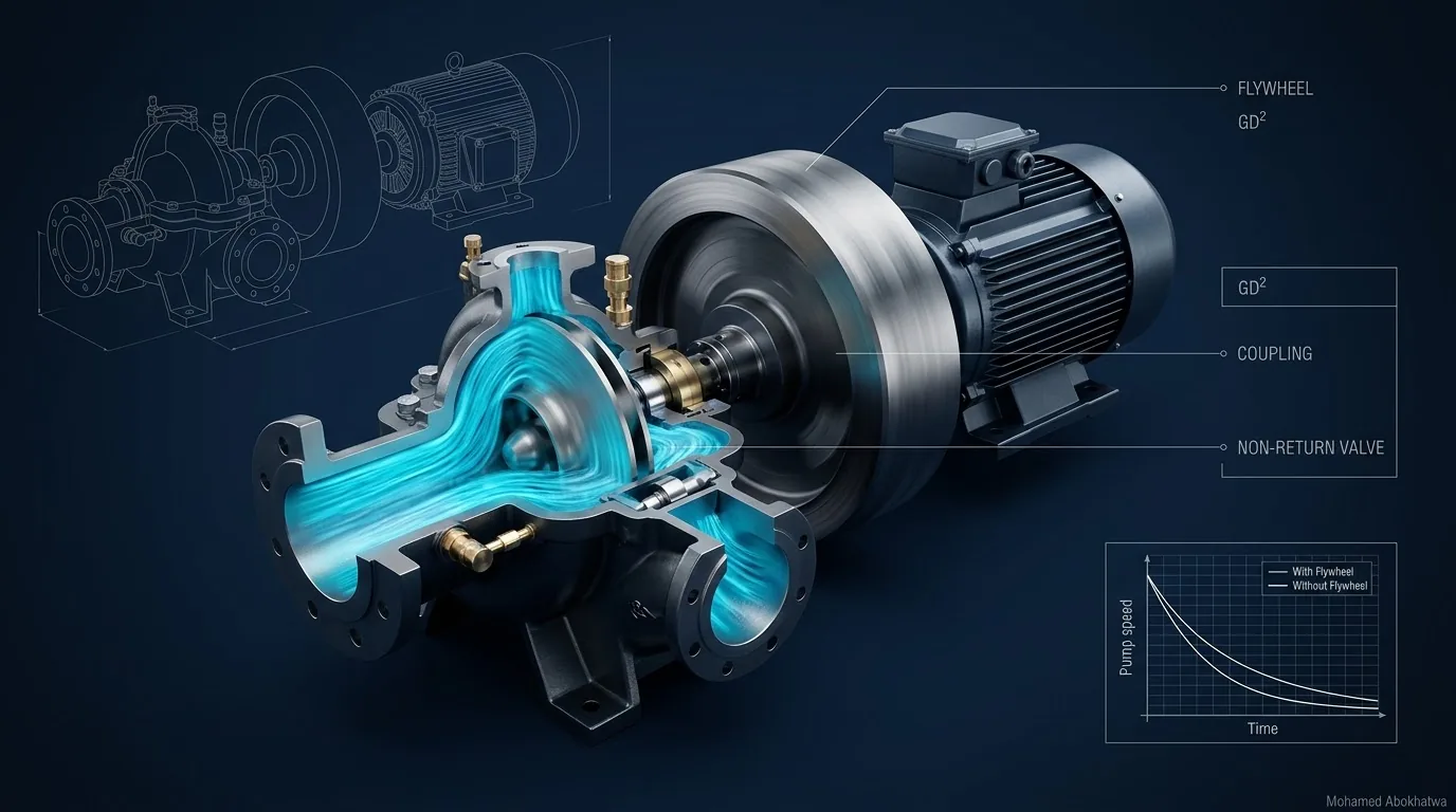
When the power fails, a pump does not stop at once. It coasts down on the energy in its rotating parts, and while it coasts it keeps the column moving. Make that rundown long enough and the downsurge never reaches vapour. On our 12 km reference main the motor and pump alone, at about 25 kg·m², protect nothing. Sixteen times that, 400 kg·m² in total, keeps every point on the line at or above +9.3 m (+7.3 m under the least favourable torque law tried), with no upsurge above the steady 85 m. The price comes at every start: with half of rated torque available for acceleration, the set takes 28.1 s to reach speed instead of 1.8.
1 · Rotating energy as surge protection
The load case that usually sizes the protection is a power failure that trips every pump at once (see Surge Scenarios in Pumping Stations). The reference main for this series is a 12 km, DN800 ductile iron K9 line [1] on a flat profile. It carries 2,520 m³/h (1.39 m/s) from an HGL of 85.0 m at the pump to 44.8 m at the reservoir, with a wave speed of 1,050 m/s. The pipe is PN16 (136 m allowable) [2], and the design minimum for this series is +3.0 m. Unprotected, with the pump modelled as stopping at once, the downsurge reaches vapour (−9.8 m) along the line, and the peak when the cavities collapse is 165–190 m. That is above PN16 whichever cavity model you believe.
A hydropneumatic vessel, a one-way surge tank or air valves put water or air back into the line. A flywheel goes after the cause instead: the column is being stopped too quickly. Until the first reflection returns from the reservoir, each cubic metre per second the pump stops delivering drops the head at the pump by
So losing all 0.70 m³/s within 2L/a = 22.9 s would call for a 149.1 m drop, from a head of 85 m that can fall only 94.8 m before it reaches vapour [3]. A pump with enough rotating mass is still delivering when the reflections come back, and the head never reaches vapour. Nothing is added to the line, there is no gas to maintain and nothing to switch on: the protection acts on every trip [4].
2 · The rundown equation: stored energy, τ and GD²
Once the motor loses its supply, the only thing driving the pump is the kinetic energy of everything on the shaft: impeller, rotor, coupling and flywheel [3][5]:
Here \(I\) is the total inertia on the shaft (kg·m²), \(\omega\) the speed, \(Q\) and \(H_p\) the flow and head the pump is still producing, \(\eta\) its efficiency and \(T_{loss}\) the windage and friction torque. Pump head falls with the square of speed. On the model pump the zero-flow head is \(100\,w^2\) metres above a 5 m suction, where \(w\) is the speed ratio. So once the speed has dropped by about 11 % (\(5 + 100\,w^2 = 85\) at \(w\) = 0.89), the pump cannot hold 85 m even at zero flow. A flywheel does not keep the pressure up. It keeps the flow going while the pressure falls.
\(E_k\) is the energy stored at running speed \(\omega_0\), and \(\tau\) is how long that energy could supply the rated power \(P_0\). At a constant rated torque \(T_0 = P_0/\omega_0\), the set would stop in \(I\omega_0/T_0 = 2\tau\). In reality the torque falls with speed and the rundown tails off more slowly, but \(\tau\) still puts sets of any speed and power on one scale [6]. Parmakian's classical charts for power failure at a pump rest on the same idea, a parameter that sets the rotor's stored energy against the pipeline's wave travel time [7].
Many data sheets give GD², which in kg·m² is numerically \(4I\). US data sheets give WR² in lb·ft², which is \(I\) itself; multiply by 0.0421 to get kg·m². A mix-up here is a factor of four in the input that matters most.
3 · The model, and six inertias on the reference main
The numbers come from a method-of-characteristics model with a vapour cavity model, cross-checked with a gas cavity model and an independent second code [3][8]. The pump is a screening model. None of this is Bentley HAMMER output: a project has to be run in HAMMER, or an equivalent program, on the real profile with the real pump data.
- Duty. 0.70 m³/s at 80 m pump head on a 5 m suction, 1,480 rpm (\(\omega_0\) = 155.0 rad/s), efficiency 0.80. That gives 685 kW of shaft power and a rated torque of 4,420 N·m.
- Pump. A simplified homologous rundown [9], \(H = 100\,w^2 - 40.8\,Q^2\), with the hydraulic torque above plus windage (2 % of rated at full speed) and an ideal non-return valve. After the valve closes we assume a churning torque of 45 % of rated at full speed, scaled with \(w^2\). Speed is integrated with the trapezoidal rule.
- Line and set. 120 reaches, 150 s runs. The bare-set inertia of 25 kg·m² is an assumption for a 685 kW four-pole set; take project values from the data sheets.
HAMMER describes the pump by four-quadrant characteristics [5][10], which set the torque during the rundown. The simple torque law used here is the main uncertainty, and section 5 puts a number on it. There is also a quirk: once its head rise has fallen to zero, the slowing model pump still passes water from its 5 m suction but takes no hydraulic torque. The bare set's speed therefore levels off at about 0.2 instead of reaching zero, and as \(I\) falls towards zero the model does not become exactly an instantaneous stop. Read that part of the speed trace as a feature of the torque law, not a prediction.
| Total I (kg·m²) | GD² (kg·m²) | Ek (MJ) | τ (s) | τ / (2L/a) | Start time (s) |
|---|---|---|---|---|---|
| 25 (bare set) | 100 | 0.30 | 0.44 | 0.02 | 1.8 |
| 100 | 400 | 1.20 | 1.75 | 0.08 | 7.0 |
| 200 | 800 | 2.40 | 3.51 | 0.15 | 14.0 |
| 400 | 1,600 | 4.80 | 7.01 | 0.31 | 28.1 |
| 800 | 3,200 | 9.61 | 14.03 | 0.61 | 56.1 |
| 1,600 | 6,400 | 19.22 | 28.05 | 1.23 | 112.2 |
| Total I (kg·m²) | Lowest head on the line (m) | Where | Lowest head at the pump (m) | Highest head on the line (m) | Speed ratio at 5 / 10 / 22.9 s |
|---|---|---|---|---|---|
| 25 | −9.8 (vapour) | 7.4–11.3 km | +2.5 | not quoted (cavitating) | 0.22 / 0.22 / 0.20 |
| 100 | −8.7 | 7.8 km | −1.3 | 88.2 (indicative) | 0.40 / 0.27 / 0.25 |
| 200 | −1.5 | 5.6 km | +5.1 | 85.0 | 0.58 / 0.40 / 0.28 |
| 400 | +9.3 | 3.0 km | +10.8 | 85.0 | 0.73 / 0.57 / 0.37 |
| 800 | +17.8 | at the pump | +17.8 | 85.0 | 0.85 / 0.73 / 0.54 |
| 1,600 | +26.0 | at the pump | +26.0 | 85.0 | 0.92 / 0.85 / 0.70 |
At 100 kg·m² the line stays only 1.1 m clear of vapour, with a small upsurge to 88.2 m at the pump. Under the least favourable torque law tried (section 5) it reaches vapour, so treat both figures as indicative. With a short rundown the lowest point is well down the line; with a long one it moves back to the pump.
4 · Interactive: the rundown
Pick an inertia and watch the pump slow down and the head at the pump respond. The grey traces are the bare motor and pump.
At 400 kg·m² the speed ratio is 0.73 at 5 s, 0.57 at 10 s and 0.37 at 2L/a. The pump-end head bottoms out at +10.8 m just as the first reflection returns, the line never drops below +9.3 m, and nothing rises above 85 m. Switch to 25 kg·m²: the speed is down to 0.22 within 5 s (where this model holds it; see section 3) and the pump-end head is below 10 m within two seconds. The pump end holds at a few metres only because the slowing pump still passes water from its suction; meanwhile the far end of the line goes to vapour. Now try 200 kg·m². The pump-end trace never falls below +5 m, yet the line fails at 5.6 km. Judge the design on the minimum envelope along the whole line, not on the history at the pump.
5 · Worked example: how much inertia the 12 km main needs
This is the sequence we follow on a project, run here on the reference main.
Step 1: the duty and the set
Step 2: test the bare set
With 25 kg·m², \(E_k\) = ½ × 25 × 155.0² = 0.30 MJ and \(\tau\) = 0.44 s, a ratio of 0.02 to 2L/a. The speed is down to 0.22 within five seconds, and the line reaches vapour over about 4 km, from 7.4 to 11.3 km. The motor and pump alone protect nothing.
Step 3: double the inertia until the whole line passes
The response is far from linear. At 100 kg·m² the lowest head is −8.7 m at 7.8 km. At 200 the pump reads +5.1 m, but the line reaches −1.5 m at 5.6 km, with about 7 km of it below +3.0 m. At 400 the whole line holds at +9.3 m or better, with the lowest point at 3.0 km, and nothing rises above 85 m. That is 16 times the bare set. The true threshold lies somewhere between 200 and 400; we design at the tested value that passes with margin.
Step 4: check that the answer survives the torque law
The weakest assumption is the torque law, so the audit reran the same line with other plausible torque characteristics. The tables above use the law that gives the highest minima of those tried. The minima moved by 2–3 m: about −4 to −1.5 m at 200 kg·m² (failing under every law tried), +7.3 to +9.3 m at 400 (passing under every law tried) and +24 to +26 m at 1,600. The conclusion is robust; the decimals are not. At worst, 400 kg·m² still clears +3.0 m by more than 4 m.
Step 5: check the pressure side, and compare
The maximum is 85.0 m: no upsurge at all, and far inside 136 m. The reference vessel used across this site (20 m³ shell, 3.5 m³ gas, DN400 differential connection) gives +4.3 m and 119.2 m on the same line with the pump stopped at once, so the comparison is not strictly like for like; even at +7.3 m the flywheel keeps more margin on the downsurge. Cost, space and operation are compared in Choosing surge protection on one pipeline.
Step 6: turn the inertia into steel
The flywheel must add 375 kg·m², which stores 4.50 MJ. For a solid steel disc \(I = \tfrac12\rho\pi t\,r^4\), so at \(t\) = 120 mm:
At 0.71 m the disc is 1.42 m across and weighs 1,492 kg. It adds 376 kg·m², for a total of 401 kg·m², and its rim runs at 110.0 m/s.
Step 7: price the start
With 50 % of rated torque available for acceleration (section 8), the start time rises from 1.8 s to 28.1 s. That figure goes to the motor manufacturer before anything else is fixed.
τ against 2L/a: a screening indicator, not a rule
Protection arrived at τ ≈ 7 s, about a third of 2L/a (0.31); at 0.15 it failed. Do not turn that into a rule. The ratio a line needs depends on its profile, friction, pump curve, torque characteristic and criterion, and a knee can separate whatever the ratio. Use it only to decide whether a flywheel is worth modelling at all [6][7].
6 · Interactive: inertia against minimum pressure
These are the six runs: minima on the line and at the pump against total inertia, with τ on the right-hand axis, and below them the minimum envelope along the main for the selected case. Set your own criterion.
At +3.0 m the smallest tested inertia that passes is 400 kg·m², with τ/(2L/a) = 0.31. Select 200 and the two minima split apart: +5.1 m at the pump but −1.5 m at 5.6 km, with about 7 km of line below the criterion. Lower the criterion to 0 m and 400 is still needed; at −1.5 m, 200 passes. Raise it to +10 m and the answer doubles to 800. Treat any pass by less than 2–3 m with suspicion, since that is the spread from the torque law alone. Up to 100 kg·m² the line is at or near vapour. From there each doubling of inertia raises the line minimum by 7–11 m (8.2 m from 800 to 1,600), but it also doubles the start time, so every extra metre of margin costs more seconds at every start.
7 · Designing the flywheel
For a solid steel disc (\(\rho\) = 7,850 kg/m³):
Inertia goes with the fourth power of radius. Doubling the thickness doubles both inertia and mass, while adding 19 % to the radius doubles the inertia for only 41 % more mass. The energy per kilogram depends only on rim speed. Rim speed sets the stress in the disc, the hub and the shaft fixing, so it is what limits the diameter, and that limit comes from the manufacturer, not from a rule of thumb.
| Disc r × t | Mass (kg) | Disc I (kg·m²) | Disc GD² (kg·m²) | Rim speed (m/s) | Total I (kg·m²) | τ (s) | Start (s) |
|---|---|---|---|---|---|---|---|
| 0.60 m × 100 mm | 888 | 160 | 639 | 93.0 | 185 | 3.24 | 13.0 |
| 0.71 m × 120 mm (design) | 1,492 | 376 | 1,504 | 110.0 | 401 | 7.03 | 28.1 |
| 0.80 m × 120 mm | 1,894 | 606 | 2,424 | 124.0 | 631 | 11.06 | 44.3 |
| 1.00 m × 150 mm | 3,699 | 1,850 | 7,398 | 155.0 | 1,875 | 32.87 | 131.5 |
In our practice, these items decide whether the flywheel gets built:
- Where it goes. On a horizontal set the disc sits between motor and pump, or on a second shaft extension at the motor's non-drive end, which needs a motor built for it. Either choice sets the baseplate length.
- Bearings and shaft. Heavy discs often get pedestal bearings of their own. The added mass lowers the critical speed of the shaft line, and the set supplier has to check it.
- Coupling. It carries flywheel torque into the pump on every trip and out of the motor on every start.
- Guarding and balancing. The disc needs a fixed guard, dynamic balancing and a positive fixing to the shaft.
- Vertical sets. The disc hangs on the thrust bearing. On vertical turbine and submersible pumps a flywheel is rarely practical.
- Space and lifting. A 1.42 m, 1.5 tonne disc changes the crane capacity, the withdrawal space and the spacing between sets.
8 · The motor start penalty
Whatever the flywheel gives back on a trip, the motor must put in on every start:
Here \(f\) is the average fraction of rated torque left over to accelerate the rotor: motor torque minus the pump's load torque. Taking \(f\) = 0.5 is our screening assumption, not a motor constant. At \(f\) = 0.5 the start takes 4τ: 1.8 s for the bare set, 7.0 s at 100 kg·m², 28.1 s at 400 and 56.1 s at 800.
- Rotor heating. The heat the rotor absorbs during a start grows with the energy being stored. The motor manufacturer must confirm the starting class, the permitted starts per hour and the minimum time between starts for the actual load inertia.
- Direct-on-line starting. The starting current and the voltage dip last for the whole run-up. Stall and overcurrent protection must allow it, and any standby generator must carry it.
- Soft starters. They cut torque along with voltage, which lowers \(f\). With a large flywheel a soft starter may not bring the set up to speed within the motor's thermal limits.
- Variable-speed drives. A drive gives near-rated torque without inrush, so \(f\) can be higher. But the drive must be rated for the duty, a controlled stop has to dissipate the stored energy or let it coast out, and a power failure trips the set exactly as before.
9 · Interactive: flywheel and motor calculator
Size a disc for your own set. The chart plots τ and start time against total inertia, with your set marked on both lines.
The default disc, 0.8 m × 120 mm, weighs 1,894 kg and adds 606 kg·m². That makes 631 kg·m² in total, 7.58 MJ stored, τ = 11.06 s, a 44.3 s start and a rim speed of 124.0 m/s, which is more than the main needs. Drag the radius to 0.71 m: the disc drops to 1,492 kg and 376 kg·m², the total is the design 401 kg·m², and the start takes 28.1 s. Raise the torque available to accelerate to 100 % and the start halves to 14.1 s. Switch to 2,960 rpm and the same disc stores four times the energy, but its rim speed doubles to 248.0 m/s, well beyond the discs of section 7; get the permissible rim speed from the manufacturer.
10 · When a flywheel is the wrong answer
Flywheels belong on short and medium-length mains, where a modest addition of inertia buys a rundown long enough to matter over the wave period [5][6][11]. Outside that range the answer is usually something else.
- Long lines. The rundown a line needs grows with its wave period. Since the start time is \(2\tau/f\), a line that needs τ to be a sizeable fraction of 2L/a needs a start time of the same order as 2L/a. On long mains that inertia soon exceeds what a motor can accelerate within its thermal limits, or what the shaft and bearings can carry [6][11]. In our practice a vessel usually scales better.
- Frequent starts. Every start pays the thermal price of section 8, and stations that cycle on level control use up their permitted starts.
- Variable-speed stations. A large flywheel works against controlled ramping and adds drive duty. The drive itself does nothing for a power-failure trip, so the surge case is the same as for a fixed-speed set.
- Knees and high points. A flywheel acts at the pump, and a knee can still separate. See One-way surge tanks at the knee.
- Upsurge problems. It does not help with a valve closure elsewhere on the system. It delays the flow reversal at the pump's non-return valve, but that valve must still close without slamming.
- Vertical and submersible sets. There is rarely anywhere to put the disc.
A surge relief valve covers only the pressure side. The full comparison is in Choosing surge protection on one pipeline.
11 · Setting it up in Bentley HAMMER
This is how we check a flywheel in HAMMER [10]; the general transient workflow and common pitfalls are covered separately. Field names differ slightly between HAMMER versions.
- Build the line and check the steady state. Model a Reservoir for the wet well, the Pump, Pipes with Junctions along the route, and a delivery Reservoir (see boundary conditions). Set wave speeds with the Wave Speed Calculator (see Wave speed), and confirm the steady HGL (85.0 m and 44.8 m here) first.
- Define the pump. Enter the duty, pump curve, efficiency and speed (1,480 rpm). Select the 4-quadrant characteristic curves from the specific speed closest to the real impeller, or ask the manufacturer for the complete characteristics; the rundown torque is where the answer is sensitive.
- Enter the inertia (pump and motor) as the total on the shaft: rotor, impeller, coupling and flywheel. Check whether each value is \(I\), GD² or WR², and whether the pump value includes the water in the impeller. Before data sheets exist, estimate the inertia from published correlations with power and speed [6], and record the estimate as an assumption.
- Set the pump trip (shut down) at the start of the run, with every pump in the station tripping together.
- Model the check valve on the pump, first as ideal and then with its real closure time/delay. A valve that closes slowly passes reverse flow before it seats and can then slam; check the reverse velocity at closure with the real closure time, even though the flywheel delays the reversal.
- Set up each inertia as its own alternative and scenario (the six inertias of the tables, 25 to 1,600 kg·m²), changing nothing else, so the envelopes can be compared and the threshold bracketed.
- Set the transient run options. Make the run duration several times 2L/a (150 s here). Accept the time step computed from the shortest pipe and the wave speeds, and check that the wave speed adjustment tolerance has not moved any wave speed materially. Turn on vapour pressure / column separation, and keep the friction method the same in every run.
- Read the time histories in the Transient Results Viewer: head and pump speed at the pump. A set that stops in about a second when you expected a slow rundown usually has its inertia in the wrong unit.
- Read the profile, not the pump. Plot the profile (path) with maximum and minimum head envelopes. Check the lowest head and its chainage against +3.0 m and the maximum against 136 m, and use the animation to see where the minimum forms.
- Test the sensitivity. Rerun the chosen inertia with neighbouring specific-speed characteristics, the lowest credible inertia and the wave speed range. If the minimum moves by more than your margin, the design is not yet robust.
- Close the loop on site. In our practice a recorded trip after commissioning is the best check of the modelled inertia; see SCADA records in transient analysis.
12 · Design checklist
- Model the unprotected case first with data-sheet inertia, and confirm that the downsurge is the problem.
- Get the inertia unit right (\(I\), GD² or WR²) for the motor, the pump and the coupling.
- Screen with Ek, τ and τ/(2L/a), and never treat the ratio as a rule.
- Double the inertia step by step and judge each case on the minimum envelope along the whole line.
- Bracket the torque-law uncertainty, and keep a margin larger than the spread (2–3 m here).
- Make sure the chosen design never reaches vapour, so that no result rests on a collapse peak.
- Confirm the maximum against the allowable pressure, and check non-return valve closure with its real characteristic.
- Size the disc from \(I = \tfrac12\rho\pi t r^4\), and get the permissible rim speed, balancing and shaft fixing from the manufacturer.
- Send the total load inertia and starting method to the motor manufacturer, and get back the start time, the thermal check and the permitted starts per hour.
- Check the electrical side: protection settings, voltage dip and any standby generator.
- Resolve the layout: bearings, coupling, guard, baseplate, crane and withdrawal space.
- Weigh the alternatives on the same line, including how often the station starts and the consequence of a protection failure.
- Run the final design in HAMMER on the surveyed profile, and verify it with a recorded trip.
- Wave speed: the number that sets the surge
- The differential orifice: empty freely, refill slowly
- Bladder, diaphragm or air-over-water vessel
- One-way surge tanks at the knee
- Surge relief valves: what a valve at the pump can protect
- Pump inertia and the flywheel
- Choosing surge protection on one pipeline
References & standards
- ISO 2531 Ductile iron pipes, fittings, accessories and their joints for water applications — the DN800 K9 ductile iron pipe of the reference main.
- EN 805 Water supply — Requirements for systems and components outside buildings — design and allowable pressures, and the surge allowance the maximum is checked against.
- Wylie, E.B. & Streeter, V.L. Fluid Transients in Systems. Prentice Hall, 1993 — the Joukowsky relation, the method of characteristics, pump boundary conditions with rotor inertia, and the discrete vapour cavity model.
- Boulos, P.F., Karney, B.W., Wood, D.J. & Lingireddy, S. “Hydraulic transient guidelines for protecting water distribution systems.” Journal AWWA, 97(5), 2005 — overview of transient control strategies, including added pump inertia.
- Chaudhry, M.H. Applied Hydraulic Transients, 3rd ed. Springer, 2014 — pump rundown equations, complete (four-quadrant) pump characteristics, and flywheels as a control measure.
- Thorley, A.R.D. Fluid Transients in Pipeline Systems, 2nd ed. Professional Engineering Publishing, 2004 — pump trip and rundown, estimating pump and motor inertia, and where flywheels are and are not practical.
- Parmakian, J. Waterhammer Analysis. Dover, 1963 — classical charts for power failure at a pump, built on pipeline and pump inertia parameters.
- Bergant, A., Simpson, A.R. & Tijsseling, A.S. “Water hammer with column separation: a historical review.” Journal of Fluids and Structures, 22(2), 2006 — column separation, vapour and gas cavity models, and why collapse peaks are model-sensitive.
- Larock, B.E., Jeppson, R.W. & Watters, G.Z. Hydraulics of Pipeline Systems. CRC Press, 2000 — homologous pump relations and transient pump boundary conditions.
- Bentley Systems. OpenFlows HAMMER product documentation and help — pump inertia, pump trip, 4-quadrant characteristic curves, check valve closure, transient run options and results viewing.
- Stephenson, D. Pipeline Design for Water Engineers, 3rd ed. Elsevier, 1989 — water hammer protection of pumping lines, and the practical limits of flywheels on long mains.