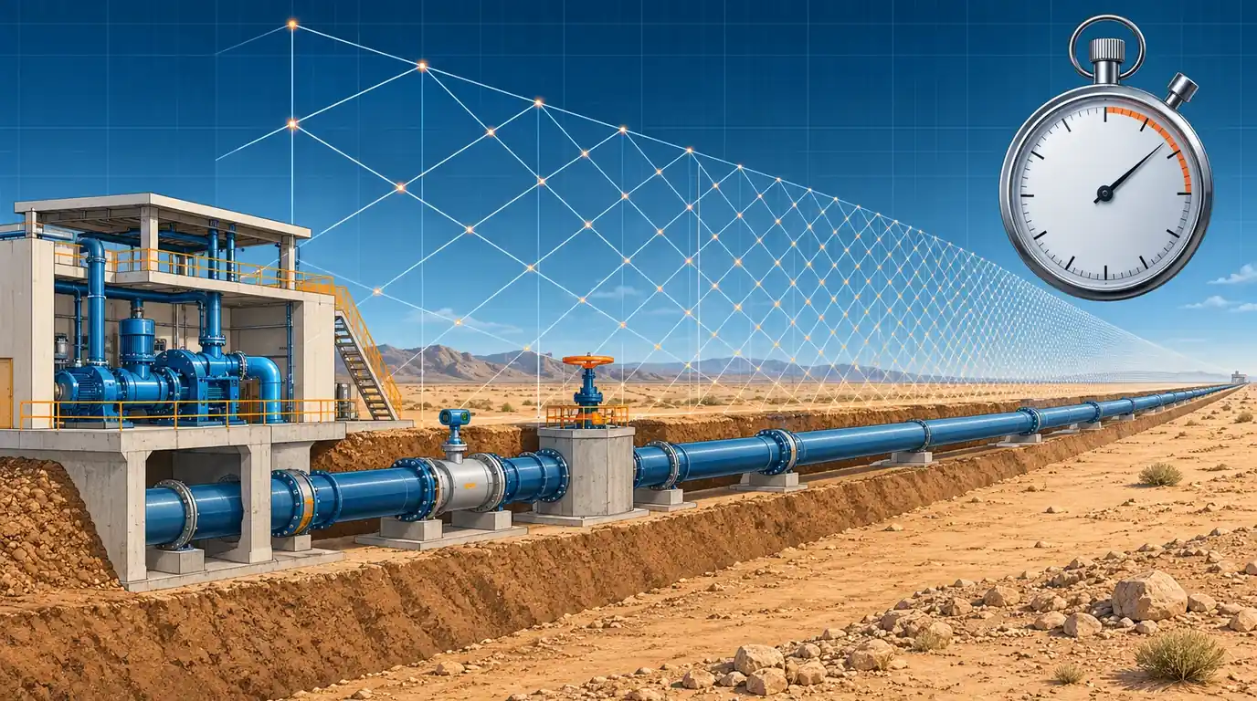
A transient model can be wrong in ways that no error message reports. We built the 12 km reference main the way it usually arrives from a GIS import, with a 2.4 m flowmeter spool and four other short pipes. We then ran it with a custom 0.1 s time step and HAMMER-style wave-speed adjustment. It reported a maximum head of 90.0 m; the converged answer is 119.3 m. At 0.05 s the same model put the line minimum at +1.4 m, below the +3.0 m design minimum used in this series, when the true value is +4.3 m, a pass. And a 90 s run of the correct model reports no upsurge at all, because the 119 m peak does not arrive until 101 s after the trip. This article sets out the five checks we make before any surge result leaves the office, with the numbers that show why each one matters.
1 · Five checks before you believe a transient run
The reference main for the surge series is a 12 km, DN800 ductile iron line carrying 0.70 m³/s (1.39 m/s) from an HGL of 85.0 m at the pump to 44.8 m at the reservoir. The wave speed is 1,050 m/s, so 2L/a = 22.9 s. Protection is a hydropneumatic vessel at the pump with 3.5 m³ of gas in a 20 m³ shell and a DN400 differential connection (see Sizing the Hydropneumatic Surge Vessel). Converged, this design keeps the line at or above +4.26 m (lowest at 4.3 km), with a maximum of 119.3 m at the pump, against a design minimum of +3.0 m and a project limit of 136 m.
Every number in this article comes from two method-of-characteristics codes written independently for this series: the solver behind the surge protection series and a new multi-pipe solver that reproduces it to 0.01 m on the uniform main [1][2]. Neither is Bentley HAMMER, but the time-step and adjustment logic follows the HAMMER documentation [3][4], so the effects shown here are the ones a HAMMER user meets. The five checks are:
- The steady state. Flows, HGL at both ends and the pump duty point match the hydraulic design before anything is tripped.
- The time step and the adjustment it forces. One time step serves the whole model, so every pipe's length or wave speed is bent to fit it. Sections 2 to 6 cover this.
- Grid convergence. Halving the time step should leave the answer unchanged (section 7).
- Run duration. The envelope must stop changing well before the run ends (section 8).
- A hand check. A test case whose answer is known, such as the Joukowsky rise for a fast valve closure, must come out right (section 9).
2 · Why one time step forces an adjustment
The method of characteristics moves along lines on which a pressure wave travels one reach in one time step. Each pipe i is cut into \(n_i\) reaches of length \(\Delta x_i = a_i\,\Delta t\), and that only works if its length is a whole number of reaches [1][5]:
With dozens of pipes of arbitrary length and several wave speeds, no practical \(\Delta t\) satisfies every pipe exactly. HAMMER therefore rounds each \(n_i\) and changes either the pipe's length or its wave speed so the rounded value fits [3][4]:
In both modes the wave takes \(n_i\,\Delta t\) to cross the pipe instead of \(L_i/a_i\). The difference lies in what else changes. Adjusting the length keeps the pipe's impedance \(a/gA\), so each metre per second of flow change still produces the right head change, but the pipe holds a different volume of water. Adjusting the wave speed keeps the volume but changes the impedance: a pipe whose wave speed is cut from 1,150 to 24 m/s responds to a flow change with 2 % of the head it should, and behaves like a small soft accumulator.
HAMMER shows the result in its Transient Time Step Options dialog: the time step, and the Max, Mean and RMS Adjustment over all pipes, in absolute terms or as a percentage. Length is the default adjustment; wave speed is offered as faster and acceptable for slow mass oscillations [3]. When the adjustment is too large HAMMER warns that the approximation “deviates excessively from the entered values”, and suggests lengthening short pipes, subdividing long ones or raising the Max Adjustment value [3]. The documentation says plainly that there is no hard rule for how much adjustment is acceptable, and that users should test the sensitivity of their results [4]. The rest of this article is that test, on one model.
3 · The model as it arrives
A model built from a GIS export or a station layout drawing carries every fitting that was drawn as a pipe. Ours has five pieces of steel station pipework between the pump and the boundary valve (one of them a 2.4 m magnetic flowmeter spool), a 3.2 m spool at a washout chamber, a 5.6 m spool at an air valve tee and a 41 m steel road crossing, among ten long ductile iron pipes. The total is still 12,000 m. The steel station pipework is thicker-walled, so we give it 1,150 m/s.
| Pipe | Description | L (m) | a (m/s) | Travel time (s) | n at 0.1 s | Length adj. at 0.1 s | Wave speed adj. at 0.1 s | n at 0.005 s |
|---|---|---|---|---|---|---|---|---|
| P-1 | Pump discharge spool | 6.5 | 1,150 | 0.0057 | 1 | +1,669 % | −94.3 % | 1 |
| P-2 | Discharge header | 11.0 | 1,150 | 0.0096 | 1 | +945 % | −90.4 % | 2 |
| P-3 | Header to vessel tee and meter | 18.4 | 1,150 | 0.0160 | 1 | +525 % | −84.0 % | 3 |
| P-4 | Flowmeter spool | 2.4 | 1,150 | 0.0021 | 1 | +4,692 % | −97.9 % | 1 |
| P-5 | Meter to station boundary valve | 27.7 | 1,150 | 0.0241 | 1 | +315 % | −75.9 % | 5 |
| P-6 | Field main | 486.0 | 1,050 | 0.4629 | 5 | +8.0 % | −7.4 % | 93 |
| P-7 | Field main | 1,212.5 | 1,050 | 1.1548 | 12 | +3.9 % | −3.8 % | 231 |
| P-8 | Field main | 834.6 | 1,050 | 0.7949 | 8 | +0.6 % | −0.6 % | 159 |
| P-9 | Washout chamber spool | 3.2 | 1,050 | 0.0030 | 1 | +3,181 % | −97.0 % | 1 |
| P-10 | Field main | 1,560.2 | 1,050 | 1.4859 | 15 | +0.9 % | −0.9 % | 297 |
| P-11 | Road crossing (steel sleeve) | 41.0 | 1,150 | 0.0357 | 1 | +180 % | −64.3 % | 7 |
| P-12 | Field main | 922.8 | 1,050 | 0.8789 | 9 | +2.4 % | −2.3 % | 176 |
| P-13 | Field main | 1,407.3 | 1,050 | 1.3403 | 13 | −3.0 % | +3.1 % | 268 |
| P-14 | Air valve tee spool | 5.6 | 1,050 | 0.0053 | 1 | +1,775 % | −94.7 % | 1 |
| P-15 | Field main | 2,015.0 | 1,050 | 1.9190 | 19 | −1.0 % | +1.0 % | 384 |
| P-16 | Field main | 1,175.9 | 1,050 | 1.1199 | 11 | −1.8 % | +1.8 % | 224 |
| P-17 | Field main to reservoir | 2,269.9 | 1,050 | 2.1618 | 22 | +1.8 % | −1.7 % | 432 |
At 0.1 s the flowmeter spool, whose true travel time is 2.1 ms, has to become one reach of 0.1 s. Adjusting length turns 2.4 m of pipe into 115 m; adjusting wave speed turns 1,150 m/s into 24 m/s. The long pipes barely move. The Mean and RMS figures look alarming only because a handful of short pipes dominate them, which is the first lesson: read the adjustment pipe by pipe, not as one number.
4 · Interactive: the adjustment for any time step
Choose the model and the adjustment mode and move the time step. The chart shows the largest adjustment in the model over the whole range of time steps for both modes; the table lists every pipe at the selected step. The readouts are the three figures HAMMER reports.
| Pipe | L (m) | a (m/s) | n | Modelled L / a | Adjustment |
|---|
On the as-imported model the largest adjustment never falls below 5 % in either mode, even at 0.001 s with 11,421 reaches for a 12 km main. The cleaned model gets below 5 % at 0.005 s with 2,284 reaches, and below 1.1 % at 0.002 s. The curves are saw-toothed: a slightly larger step can need less adjustment than a smaller one, because what matters is how close each \(L_i/a_i\Delta t\) falls to a whole number. Run effort is the number of reaches times the number of steps, relative to the same model at 0.1 s.
5 · What the adjustment does to the answer
We ran the vessel-protected trip on both models at seven time steps in both modes, 150 s each, and compared every result with a reference run of the as-imported model at 0.0005 s (22,850 reaches, largest adjustment 4.3 %). The reference gives +4.26 m at 4.3 km, a maximum of 119.27 m and a peak gas volume of 16.19 m³. The cleaned model at 0.0005 s agrees to 0.01 m.
| Δt (s) | Reaches | Min, length adj. (m) | Max, length adj. (m) | Min, wave speed adj. (m) | Max, wave speed adj. (m) |
|---|---|---|---|---|---|
| 0.2 | 65 | +2.64 | 123.07 | +12.44 | 85.00 |
| 0.1 | 122 | +3.58 | 121.43 | +4.92 | 89.95 |
| 0.05 | 234 | +4.05 | 120.07 | +1.44 | 109.69 |
| 0.02 | 575 | +4.20 | 119.52 | +4.07 | 117.57 |
| 0.01 | 1,144 | +4.25 | 119.34 | +4.18 | 118.96 |
| 0.005 | 2,285 | +4.26 | 119.29 | +4.24 | 119.21 |
| 0.002 | 5,710 | +4.26 | 119.28 | +4.25 | 119.35 |
Four things stand out.
- The errors go both ways. At 0.1 s, wave-speed adjustment reports a maximum of 90.0 m, 29 m low, and a minimum of +4.9 m, 0.7 m better than the truth. The soft spools near the pump absorb the upsurge. At 0.05 s the same mode puts the minimum at +1.4 m near 0.9 km: against the +3.0 m minimum, a design that passes is reported as failing. With a −3 m criterion this case would still pass, but the error is the same 2.8 m, and it would flip any design whose true minimum lay within 2.8 m of that criterion.
- Length adjustment fails more gently here. It keeps every pipe's impedance, so its errors come from the extra water and travel time. At 0.1 s it reads 121.4 m and +3.6 m, conservative on both sides, but still 0.7 m out on a 1.3 m margin.
- At 0.005 s and below both modes agree with the reference to within 0.1 m on both extremes. Even then the worst adjusted pipe, now a chamber spool changed by 24 %, still moves the peak at the pump by 0.08 m in wave-speed mode.
- At 0.2 s the model says there is no problem at all. Wave-speed adjustment reports a maximum of 85.0 m, the steady head, and a minimum of +12.4 m. Length adjustment at the same step reports +2.6 m, a failure. Neither number has anything to do with the real main.
Switch to the cleaned model and the spread collapses: at 0.1 s the maximum is within 1.2 m of the reference in both modes, and from 0.05 s down every result is within 0.15 m. At 0.1 s the cleaned model in wave-speed mode still drops the minimum to +3.4 m near 1 km, because the 41 m road crossing is then one reach with its wave speed cut by 64 % and the 66 m station pipe by 43 %. At 0.2 s even the cleaned model fails in wave-speed mode (−0.4 m). A large custom time step is the first thing we look for in someone else's run.
6 · Cleaning the model: what to merge and what to keep
The cure for adjustment is rarely a smaller time step. On a large network that multiplies run time, and HAMMER's documentation itself points to lengthening short pipes, subdividing long ones and using Skelebrator to remove short pipes [3][4]. We merged five things:
- Station pipework P-1 to P-5 became one 66.0 m steel pipe. Where merged pipes have different wave speeds, keep the travel time: \(a_{eq} = \sum L_i \big/ \sum (L_i/a_i)\). Where they have different bores, keep the volume and the impedance as far as you can, and keep the station in detail if a check valve or the vessel connection sits inside it.
- Chamber spools (P-9, P-14) were added to the neighbouring field pipe. A washout or air valve node must stay where the device is; only the spool goes.
- The road crossing stayed at 41 m: it is long enough to be a few reaches and its wave speed is genuinely different.
Some things must never be merged away, whatever they do to the time step: a dead-end branch (it reflects the wave and doubles the pressure at its end), a closed valve, the node of any protection device, a high point or a change of gradient on the profile, and any pipe where the diameter changes enough to change the impedance. When in doubt, keep the pipe and reduce the time step for that run only.
7 · Halve the step: grid convergence on the uniform main
Even with no adjustment at all, a coarse grid smears steep wave fronts and moves the extremes. On the uniform reference main, where any \(\Delta t = 12{,}000/(1{,}050\,N)\) fits exactly, we ran three cases at six grid sizes: the vessel design, the 400 kg·m² flywheel of Pump Inertia and the Flywheel, and the unprotected trip, whose peak comes from cavity collapse.
| Reaches N | Δx (m) | Δt (s) | Vessel: min (m) | Vessel: max (m) | Flywheel: min (m) | Unprotected max, vapour cavity (m) | Unprotected max, gas cavity (m) |
|---|---|---|---|---|---|---|---|
| 30 | 400 | 0.381 | +4.57 | 118.90 | +9.40 | 189.1 | 168.1 |
| 60 | 200 | 0.191 | +4.41 | 119.06 | +9.36 | 189.3 | 161.1 |
| 120 | 100 | 0.095 | +4.33 | 119.15 | +9.34 | 189.9 | 164.6 |
| 240 | 50 | 0.048 | +4.29 | 119.19 | +9.33 | 190.0 | 161.2 |
| 480 | 25 | 0.024 | +4.27 | 119.21 | +9.32 | 190.0 | 162.5 |
| 960 | 12 | 0.012 | +4.26 | 119.22 | +9.32 | 190.1 | 162.2 |
The two protected cases converge cleanly. From the coarsest grid to the finest, the vessel minimum falls by 0.31 m, and every halving halves the change (0.16, 0.08, 0.04, 0.02, 0.01 m), which is first-order behaviour. A model at 0.38 s would report +4.57 m and overstate the margin above +3.0 m by a quarter. The flywheel minimum hardly moves (0.08 m). The collapse peak behaves differently: the vapour cavity model settles at 189–190 m, while the gas cavity model wanders between 161 and 168 m with no trend. Collapse peaks do not converge the way a single-phase result does, which is why this series quotes them as a range and designs to keep the line out of vapour [6][7].
The extrapolated value assumes first-order convergence: \(H_\infty \approx 2H_{2N} - H_N\). From every grid, even N = 30 (0.38 s), the extrapolation lands within 0.01 m of the finest run. With a 0.10 m tolerance the vessel minimum is converged from N = 60. Select N = 960 and there is no finer run to compare with, which is the honest position for any production model: the last halving is the evidence.
In HAMMER this check is two runs: the time step HAMMER suggests, and the same scenario with Use Custom Time Step? checked and half that value. The documentation recommends the same kind of test with a very small step [4]. Compare the minimum and maximum envelopes at the critical points, not only at the pump.
8 · Run duration: the peak that arrives at 101 seconds
A pump trip on a long main with a vessel is a slow event. The first downsurge is over in one wave cycle, but the column then swings back and forth between the vessel and the reservoir with a period set by the gas volume and the length of the line, much longer than 2L/a. On the reference main the lowest head is reached at 18.6 s. The highest head, 119.2 m at the pump, comes at 101 s on the return swing, more than four times 2L/a. The HAMMER workflow article on this site uses 90 s as an example duration; on this main a 90 s run would report a maximum of 85.0 m, the steady head, and miss the upsurge entirely.
The minimum is captured from 19 s onwards; the maximum needs 102 s. Between 102 and 400 s nothing changes, so 150 s (6.6 × 2L/a) is enough here. On a main protected by air valves, a one-way tank or a flywheel the governing peak can come later still, after a cavity has grown and collapsed or a tank has drained.
Our rule: run at least long enough to see the first full swing of the slowest oscillation in the system, then extend the run by half and confirm that neither envelope moves. If the maximum or minimum occurs in the last quarter of the run, the run is too short.
9 · Hand checks the model must pass
Before trusting a model of a real system, we run a test scenario whose answer we already know. The cleanest is the Joukowsky test: replace the pump with a reservoir at the duty head, put a valve at the far end, and close it faster than 2L/a. The head at the valve must jump by [1][5]
Our test model holds 45.8 m at the valve in steady flow (1.0 m across the open valve).
| Check | Hand value | Model | Comment |
|---|---|---|---|
| Rise at the valve, instant closure (first step) | 149.1 m | 149.1 m | from 45.8 m to 194.9 m in one step |
| Head at the valve, 5 s closure, just after closure | about 195 m | 196.3 m | closure well inside 2L/a, so the full Joukowsky rise plus a little line packing |
| Peak at the valve, instant closure | ≥ 194.9 m | 233.8 m at 22.9 s | Joukowsky plus line packing, just before the reflection returns at 2L/a = 22.9 s |
| Peak at the valve, 5 s closure | ≥ 194.9 m | 227.5 m at 24.4 s | slightly lower and later: the rise is built over 5 s instead of in one step |
The rise above the Joukowsky value is line packing: as the front runs upstream it meets water at progressively higher head, and the water still flowing towards the valve behind it keeps packing the line, so the head at the valve keeps climbing until the reflection returns [1][8]. On a long, high-friction main it is a real part of the peak. If the first rise in your model is a few percent off \(a\Delta V/g\), look at the adjusted wave speeds before anything else.
Three more checks take minutes:
- Steady state. The initial HGL along the profile matches the hydraulic model, every pump sits at its duty point, and no air valve or relief valve is open at time zero.
- Travel time. A disturbance at the pump must reach chainage \(x\) at \(x/a\): 5.71 s to mid-line here. Place a report point there and look at the trace.
- Energy. With friction on, every oscillation must decay. An oscillation that grows or does not die away points to a boundary or device input error.
10 · Setting it up in Bentley HAMMER
Field names differ slightly between HAMMER versions; these follow the current documentation [3][4][9].
- Compute the steady state first and compare it with the design model: flows, pump duty points and the HGL at the ends of the main (85.0 m and 44.8 m here).
- Clean the model for transients. Merge station pipework, chamber spools and other short pipes as in section 6, or use Skelebrator, but keep every device node, dead end, closed valve and high point.
- Open Transient Time Step Options and read the suggested Time Step and the Max, Mean and RMS Adjustment. Set Adjustment Type to relative so the figures are percentages, and sort the pipe adjustments to find the worst pipes.
- Leave Adjust on Length unless you have a reason to change it, and do not raise Max Adjustment just to clear the warning. If the warning appears, fix the short pipes it points to.
- Set the run duration in time, not time steps, and make it at least 6–7 × 2L/a for a pumped main with a vessel. Extend it by half once and confirm that the envelopes do not change.
- Choose report points at the pump, at the vessel, at every high point and knee, and at mid-line, and turn on Generate Animation Data so the profile envelopes can be checked along the whole line.
- Run the halved step: check Use Custom Time Step?, enter half the suggested value, and rerun the governing scenario. Record both results in the report.
- Run the Joukowsky test once per model as a separate scenario, with the pump replaced by a reservoir and a valve closing in a fraction of 2L/a at the far end.
- Record everything: time step, adjustment mode, max/mean/RMS adjustment, the worst pipes, the halved-step result and the run duration, in the model basis of the report.
11 · Checklist
- Steady state matches the design model before any transient run.
- Short pipes merged where they carry no device, dead end, high point or change of section.
- Adjustment read pipe by pipe, with the worst pipes named and their effect understood.
- Max Adjustment left at a value you can defend, never raised only to clear a warning.
- Halved time step run on the governing scenario, with the change in minimum and maximum recorded.
- Collapse peaks quoted as a range, and the design judged on keeping the line out of vapour.
- Run duration long enough that neither envelope changes when it is extended by half.
- Joukowsky test and travel-time check passed by the model.
- Envelopes read along the whole line, not only at the pump.
- All of the above written into the report (see The Surge Study Report).
- Is your HAMMER run right? Time step, adjustment and run duration
- Pump data for a pump trip: inertia, specific speed and four-quadrant curves
- Reading the surge envelope against the pipe's real limits
- The surge study report: what to deliver and what a reviewer checks
References & standards
- Wylie, E.B. & Streeter, V.L. Fluid Transients in Systems. Prentice Hall, 1993: the method of characteristics, the Courant condition, interpolation and wave-speed adjustment, and the Joukowsky relation.
- Abokhatwa, M. Surge protection design series, abokhatwa.com, 2026: the reference main, the vessel design and the verified MOC solver used throughout this article.
- Bentley Systems. OpenFlows HAMMER documentation, “Transient Time Step Options Dialog Box”: time step, Max, Mean and RMS Adjustment, Adjust (Length or Wave speed), Adjustment Type, Use Custom Time Step and the excessive-adjustment warning.
- Bentley Systems. OpenFlows HAMMER documentation, “Selection of the Time Step”: why the time step forces adjustments, the absence of a fixed limit, and sensitivity testing with a smaller step.
- Chaudhry, M.H. Applied Hydraulic Transients, 3rd ed. Springer, 2014: discretisation of pipe networks, wave-speed adjustment and the accuracy of characteristic methods.
- Bergant, A., Simpson, A.R. & Tijsseling, A.S. “Water hammer with column separation: a historical review.” Journal of Fluids and Structures, 22(2), 2006: vapour and gas cavity models and why collapse peaks depend on the model and the grid.
- Simpson, A.R. & Bergant, A. “Numerical comparison of pipe-column-separation models.” Journal of Hydraulic Engineering, 120(3), 1994: grid sensitivity of the discrete vapour cavity model.
- Thorley, A.R.D. Fluid Transients in Pipeline Systems, 2nd ed. Professional Engineering Publishing, 2004: line packing and the effect of friction on the transient peak.
- Karney, B.W. & Ghidaoui, M.S. “Flexible discretization algorithm for fixed-grid MOC in pipelines.” Journal of Hydraulic Engineering, 123(11), 1997: the errors introduced by wave-speed adjustment and interpolation, and ways to limit them.