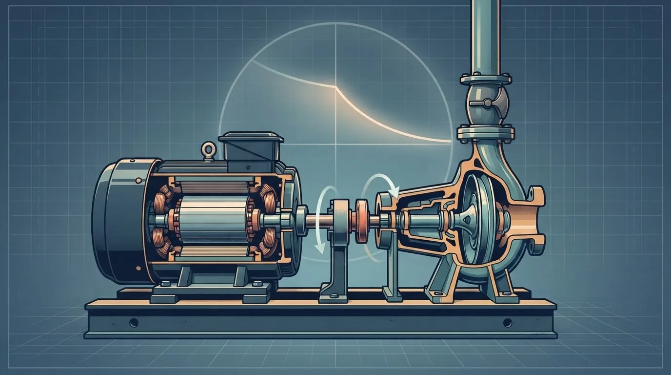
At tender stage a surge study rarely has a motor data sheet, a pump inertia or a complete pump characteristic, yet the pump trip that sizes the protection depends on all three. The usual answer is the correlation built into HAMMER's inertia calculator, which gives 44.0 kg·m² for our 685 kW, 1,480 rpm set. On a 4 km main from the same station, that estimate puts the lowest head anywhere between −0.3 and +3.2 m depending on the torque characteristic, either side of the +3.0 m criterion. At 25 kg·m² the line fails under every characteristic we tried; at 88 it passes under all of them. On the 12 km reference main the same uncertainty changes nothing: the line reaches vapour at any credible inertia. This article shows how to estimate the data, how to tell whether the estimate matters, and what to demand from the pump supplier.
1 · What the pump trip needs from the pump
After a power failure the motor torque disappears and the rotating parts slow down under the torque the water still demands from the impeller [1][2]:
Three pieces of pump data decide how that rundown goes:
- The inertia \(I\) of everything on the shaft, which sets how much energy is stored and how fast it is given up.
- The torque the pump absorbs as speed and flow fall, including the zones where flow or rotation reverse. It comes from the complete, or four-quadrant, characteristic.
- The head the slowing pump still produces, from the same characteristic, which is what the pipeline sees.
HAMMER asks for these as the pump's Inertia (Pump and Motor), its Speed and its Specific Speed, which selects a built-in four-quadrant curve [3][4]. The HAMMER workflow article shows where they are entered. This article is about where the numbers come from when nobody has given them to you.
The station is the one used throughout the surge series: 0.70 m³/s at 80 m pump head on a 5 m suction, 1,480 rpm, efficiency 0.80, which gives 685 kW of shaft power and a rated torque of 4,420 N·m. We test it on four mains of the same DN800 ductile iron line and the same friction gradient: 1, 2, 4 and 12 km long, with 2L/a from 1.9 to 22.9 s. The 12 km main is the reference main of the series [5].
2 · Estimating inertia without a data sheet
The correlations most programs use for a first estimate are attributed to Thorley and quoted in Wylie and Streeter [1][6]. HAMMER's Pump and Motor Inertia Calculator uses an empirical relation from Thorley, with the brake power at best efficiency and the speed as inputs [3]. With \(P\) in kW, \(N\) in rpm and \(I\) in kg·m²:
For our set:
The total is 44.0 kg·m², of which the motor is 86 %: the motor rotor dominates, and the impeller adds about a sixth of the motor figure here. The series so far has used 25 kg·m² as an assumed bare-set value; the correlation gives 76 % more. Neither is wrong. A correlation fitted to a population of machines describes the population, and individual motors scatter widely around it: high-efficiency and large-frame motors carry more rotor, and some users report calculator estimates several times the maker's figure for a particular set. Treat the estimate as the centre of a range, and test the range.
Two more contributions are often forgotten. The water inside the impeller rotates with it and adds to the pump inertia; manufacturers state whether their figure is “dry” or “wet”. A spacer coupling on a large set can add a few percent. On a vertical turbine pump the line shaft and every bowl assembly count.
At 685 kW and 1,480 rpm the set stores 0.53 MJ, enough to supply rated power for 0.77 s. Drop to 740 rpm at the same power and the inertia rises 3.4 times, because a slower machine for the same power is a bigger machine, yet the stored energy falls by 14 %, since it goes with the square of speed. A two-pole set at 2,960 rpm has a third of the inertia but stores 31 % more energy (τ = 1.0 s). By the correlation, speed matters less than most engineers expect: across four speeds τ stays between 0.66 and 1.0 s for this power.
3 · Specific speed and the four-quadrant curve
During a trip the pump passes through states its catalogue curve never shows: reduced speed at normal flow, zero flow while still turning, reverse flow through a forward-turning impeller and, without a check valve, reverse rotation as a turbine. The complete characteristic covers all of them, usually in the Suter form, two functions \(W_H\) and \(W_B\) of the angle \(\theta = \arctan(\alpha/v)\), where \(\alpha\) and \(v\) are speed and flow as fractions of rated [1][2][7]. Nobody measures this for a project pump. Programs carry a small library of measured characteristics, one per specific speed, and scale them to the rated point of your pump. The specific speed tells the program which shape to borrow:
In US units (rpm, gpm, ft) the same pump is 2,390. HAMMER's documentation lists typical values with built-in curves of 25, 94 and 145 in SI units (1,280, 4,850 and 7,500 in US units), and tells the user to select the closest available setting [4]; further curves in its library come from Stepanoff and from Thorley and Chaudhry [3][8][9]. Our pump at 46 sits between the radial curve at 25 and the mixed-flow curve at 94, nearer the radial one. The documentation adds two points worth repeating: the error from using the wrong curve cannot be interpolated by specific speed, so it should be bracketed by running neighbouring curves, and results are less sensitive to the choice when a check valve stops reverse flow [4].
We cannot reproduce HAMMER's library curves here, so to show what the characteristic does we use the three rundown torque laws already used in Pump Inertia and the Flywheel: constant efficiency on the head actually produced (“duty”), a law that never lets the torque fall below what the shut-off head would demand (“shut-off”), and a generic radial characteristic \(\beta/\alpha^2 = 0.45 + 0.75x - 0.2x^2\) (“radial”). Each pump has an ideal check valve. These are stand-ins for the spread between real characteristics, not substitutes for them.
The impeller-type bands are indicative: radial below about 40 (SI), mixed flow from about 40 to 160, axial above. A multistage pump is assessed per stage, which is why a high-head multistage pump often lands at a low specific speed. When a pump falls between two library curves, run both and design to the worse.
4 · Interactive: one trip, four mains
Choose a main length, an inertia and a torque law and watch the pump slow down and the head at the pump fall. The grey trace is the same main with the pump stopping instantly, the most conservative assumption a model can make.
On the 4 km main with the estimated 44 kg·m² and the radial law, the speed falls below half in 1.5 s and the line bottoms out at +1.8 m, 1.0 km from the pump. Switch to the duty law and it passes at +3.2 m; switch to the shut-off law and it fails at −0.3 m. On the 12 km main every inertia up to 88 kg·m² takes the line to vapour, or within 0.1 m of it, whatever the law: the rundown is over long before the first reflection returns at 22.9 s. On the 1 km main even 25 kg·m² keeps the line above +6.8 m. The instant-stop trace shows why nobody should design a short main on that assumption: it predicts vapour and collapse peaks of 240–295 m on the three short mains, while the estimated 44 kg·m² keeps the 1 and 2 km lines above +5 m under every law.
5 · Does the inertia estimate matter? Look at τ against 2L/a
The comparison that decides whether the pump data matter is the rundown time against the pipeline's wave period. The time constant \(\tau = E/P = I\omega_0^2/2P\) is 0.77 s for the estimated set. Set against 2L/a:
| Main | 2L/a (s) | τ/(2L/a) at 44 | Instant stop | I = 25 | I = 44 | I = 88 | I = 176 |
|---|---|---|---|---|---|---|---|
| 12 km | 22.9 | 0.03 | vapour | vapour | vapour | vapour to −9.8 | −5.7 to −3.0 |
| 4 km | 7.6 | 0.10 | vapour | −2.6 to +0.9 | −0.3 to +3.2 | +4.4 to +7.5 | +15.4 to +17.0 |
| 2 km | 3.8 | 0.20 | vapour | +1.4 to +5.0 | +5.0 to +7.8 | +16.1 to +17.4 | +27.3 to +30.1 |
| 1 km | 1.9 | 0.41 | vapour | +6.8 to +9.2 | +16.4 to +17.7 | +28.3 to +31.0 | +40.3 to +43.3 |
- Long main, small ratio (12 km, τ/(2L/a) = 0.03). The pump is effectively stopped before the line knows anything about it. Inertia between 25 and 88 kg·m² changes nothing, the line reaches vapour and protection is needed. Model the real inertia anyway, but do not chase the data.
- Middle ground (4 km, ratio 0.10). The answer depends on both the inertia and the characteristic. At the estimate, the three laws straddle the criterion. This is where a wrong guess changes the design, and where a vendor's inertia and four-quadrant data earn their cost.
- Short main, larger ratio (1–2 km, ratio 0.2–0.4). Inertia alone protects the line at the estimated value. The instant-stop assumption would buy protection that is not needed.
The upsurge tells the same story. On the 4 km main the maxima stay between 129 and 135 m for every inertia up to 88 kg·m² and every law, close to the 136 m project limit used in this series, so the upsurge check needs the same care as the downsurge.
“Decision at the estimate” compares the worst and best law at 44 kg·m² with the criterion: if both pass, the estimate is good enough; if both fail, protection is needed whatever the data say; if they disagree, get the data. On the 4 km main at +3.0 m the laws disagree. Lower the criterion to 0 m and the decision still depends on the data. On the 12 km main the smallest tested inertia that passes all three laws at +3.0 m is the 400 kg·m² flywheel case.
6 · With a vessel: is the instant stop conservative?
Many analysts model the pump as stopping instantly when sizing a vessel, on the grounds that it is conservative. On the 12 km main we sized the vessel gas volume (differential DN400 connection, shell 5.7 times the gas, +3.0 m everywhere) for each assumption:
| Pump model | Constant efficiency (duty) | Generic radial | Shut-off floor |
|---|---|---|---|
| Instant stop | 3.22 | ||
| I = 25 kg·m² | 3.20 | 3.21 | 3.20 |
| I = 44 kg·m² (estimate) | 2.72 | 3.19 | 2.72 |
| I = 88 kg·m² | 2.19 | 3.13 | 2.19 |
With the generic radial law, real inertia saves at most 3 % of gas. Under the two laws in which the slowing pump keeps delivering longer, the estimated set saves 15 % and twice the estimate 32 %. The instant stop is conservative in every case and costs up to half as much gas again (3.22 against 2.19 m³); on a long main that is a small price for not depending on data you do not have. On short mains, where section 5 showed inertia doing most of the work, the instant stop can oversize a vessel many times over or call for one that is not needed at all, and real data pay for themselves. The same caution applies to the upsurge: the pump's rundown changes when the check valve closes and how fast the reverse flow builds, which is covered in check valve slam.
7 · Reverse flow, reverse rotation and the check valve
Once the pump's head falls below the line head, the flow at the pump reverses. With a check valve that closes cleanly, the pump simply runs down. Without one, or with a valve that closes late, water flows back through the pump, stops it, and then drives it backwards as a turbine towards its runaway speed [1][2][7]. That is where the four-quadrant data matter most, and where results become very sensitive to the curve chosen [4]. Three practical points:
- Reverse rotation. Ask the manufacturer for the runaway speed in reverse at the maximum static head, and whether the pump, motor bearings and coupling may spin backwards. Some motors must not be restarted while turning backwards, which sets an interlock on the restart time.
- Anti-reverse devices. A ratchet stops reverse rotation and turns the pump into a fixed restriction to reverse flow; the model must then treat the pump as locked, not free-wheeling.
- Check valve timing. The inertia sets how soon the flow reverses, so it also sets the reverse velocity a slow valve meets. A larger inertia delays reversal and usually softens the slam.
8 · Worked example: from no data to a defensible pump model
Step 1: the duty and power
Step 2: estimate the inertia and set a range
Correlation: 37.7 + 6.3 = 44.0 kg·m². With ±50 % the range to test is 22–66 kg·m². We ran 25, 44 and 88 to cover it with margin. Stored energy at the estimate: \(\tfrac12 \times 44.0 \times 155.0^2 = 0.53\) MJ; \(\tau\) = 0.77 s.
Step 3: specific speed and characteristic
\(N_s\) = 46 (SI), a radial impeller. In HAMMER we select the closest typical value (25) and repeat the governing run with the mixed-flow curve (94) to bracket the characteristic, as the documentation advises [4].
Step 4: compare τ with 2L/a
For the 4 km main: 0.77/7.62 = 0.10. That is in the zone where the data matter, so the trip has to be run across the whole range of inertia and characteristic, not at one point.
Step 5: run the bracket and read the decision
At 25 kg·m² the minimum is −2.6 to +0.9 m (fails under every law); at 44, −0.3 to +3.2 m (undecided); at 88, +4.4 to +7.5 m (passes under every law). The design cannot be fixed on estimates.
Step 6: decide
Either protect the main on the conservative side (a small vessel or a flywheel, sized at 25 kg·m² and the shut-off law), or make the pump data a hold point: specify the minimum total inertia the motor and pump must provide, and require the supplier's inertia and complete characteristics before the protection is frozen. On the 4 km main a total of 88 kg·m² passes under every law tried, so a specification can simply require it, with a small flywheel if the chosen motor falls short (see Pump Inertia and the Flywheel).
9 · What to demand in the pump specification
Most surge studies stall at detailed design because the pump package arrives without the transient data. We write these into the pump and motor specification, with the surge study named as their user:
- Moment of inertia of the motor rotor, the pump rotor with entrained water, the coupling and any flywheel, each stated as \(I\) in kg·m² (state explicitly if GD² or WR² is given).
- Complete performance curves from shut-off to run-out at rated speed: head, power, efficiency and NPSH required, with the duty point and best efficiency point marked.
- Specific speed and impeller type, and the complete (four-quadrant) characteristics in Suter or equivalent form where the manufacturer has them for the impeller design or a geometrically similar one.
- Reverse running: whether reverse rotation is permitted, the runaway speed at the maximum reverse head, and the maximum time at runaway.
- Motor starting data: the maximum load inertia the motor can accelerate, the starting time with the specified starter, and permitted starts per hour.
- Check valve type and dynamic characteristic (reverse velocity against deceleration), from the valve manufacturer.
- A minimum total inertia, where the surge study shows the line depends on it, as a performance requirement with a test or certificate.
10 · Setting it up in Bentley HAMMER
Field names differ slightly between versions; these follow the current documentation [3][4][10].
- Enter the pump curve and efficiency for steady state, and confirm the duty point and power in the steady run.
- Open the pump's transient properties and enter the Speed (Full) in rpm.
- Inertia (Pump and Motor): enter the vendor value if you have it. If not, use the Pump and Motor Inertia Calculator with the brake power at best efficiency and the speed, and record the result as an assumption. Check whether a vendor value is \(I\), GD² or WR² before typing it in.
- Specific Speed: calculate it per stage at best efficiency and select the closest available value. Note it in the assumptions register.
- Pump trip: set the pump to shut down at the start of the run (all pumps together for the power-failure case), and model the check valve as described in the check valve article.
- Make the bracket explicit: create alternatives for the low, estimated and high inertia and for the neighbouring specific-speed curve, and a scenario for each combination, changing nothing else.
- Compare the envelopes along the whole line, and report the range. If the decision changes inside the range, say so and make the pump data a hold point.
- Replace estimates with vendor data as soon as they arrive, rerun, and keep both runs in the report.
11 · Checklist
- Inertia source recorded: vendor (with the document) or correlation (with the inputs).
- Units checked: \(I\), GD² or WR², wet or dry, coupling included.
- Range tested around any estimate, at least ±50 %.
- Specific speed calculated per stage, closest curve used and a neighbouring curve run as a bracket.
- τ/(2L/a) worked out to judge whether the pump data matter.
- Instant stop compared with the real rundown, and the conservative choice explained.
- Reverse flow and rotation considered, with the check valve modelled realistically.
- Pump data written into the specification as a hold point where the decision depends on it.
- Is your HAMMER run right? Time step, adjustment and run duration
- Pump data for a pump trip: inertia, specific speed and four-quadrant curves
- Reading the surge envelope against the pipe's real limits
- The surge study report: what to deliver and what a reviewer checks
References & standards
- Wylie, E.B. & Streeter, V.L. Fluid Transients in Systems. Prentice Hall, 1993: pump boundary conditions with rotor inertia, complete pump characteristics in Suter form, and inertia correlations for motors and pumps.
- Chaudhry, M.H. Applied Hydraulic Transients, 3rd ed. Springer, 2014: pump rundown equations, four-quadrant characteristics, reverse flow and reverse rotation.
- Bentley Systems. OpenFlows HAMMER documentation, “Pump and Motor Inertia Calculator” and pump transient properties: inertia from brake power at best efficiency and speed, using an empirical relation by Thorley.
- Bentley Systems. OpenFlows HAMMER documentation, “Specific Speed”: definition, the typical values 25, 94 and 145 (SI) with built-in curves, selecting the closest value, bracketing, and the effect of a check valve.
- Abokhatwa, M. Surge protection design series, abokhatwa.com, 2026: the 12 km DN800 reference main, its pump station and the verified MOC solver.
- Thorley, A.R.D. Fluid Transients in Pipeline Systems, 2nd ed. Professional Engineering Publishing, 2004: pump trip and rundown, and estimating pump and motor inertia from power and speed.
- Larock, B.E., Jeppson, R.W. & Watters, G.Z. Hydraulics of Pipeline Systems. CRC Press, 2000: homologous relations and transient pump boundary conditions.
- Stepanoff, A.J. Centrifugal and Axial Flow Pumps, 2nd ed. Wiley, 1957: specific speed, impeller types and complete pump characteristics.
- Thorley, A.R.D. & Chaudry, A. “Pump characteristics for transient flow analysis”: cited in the HAMMER documentation as the source of further predefined four-quadrant curves.
- Boulos, P.F., Karney, B.W., Wood, D.J. & Lingireddy, S. “Hydraulic transient guidelines for protecting water distribution systems.” Journal AWWA, 97(5), 2005: data needs and pump modelling in transient studies.