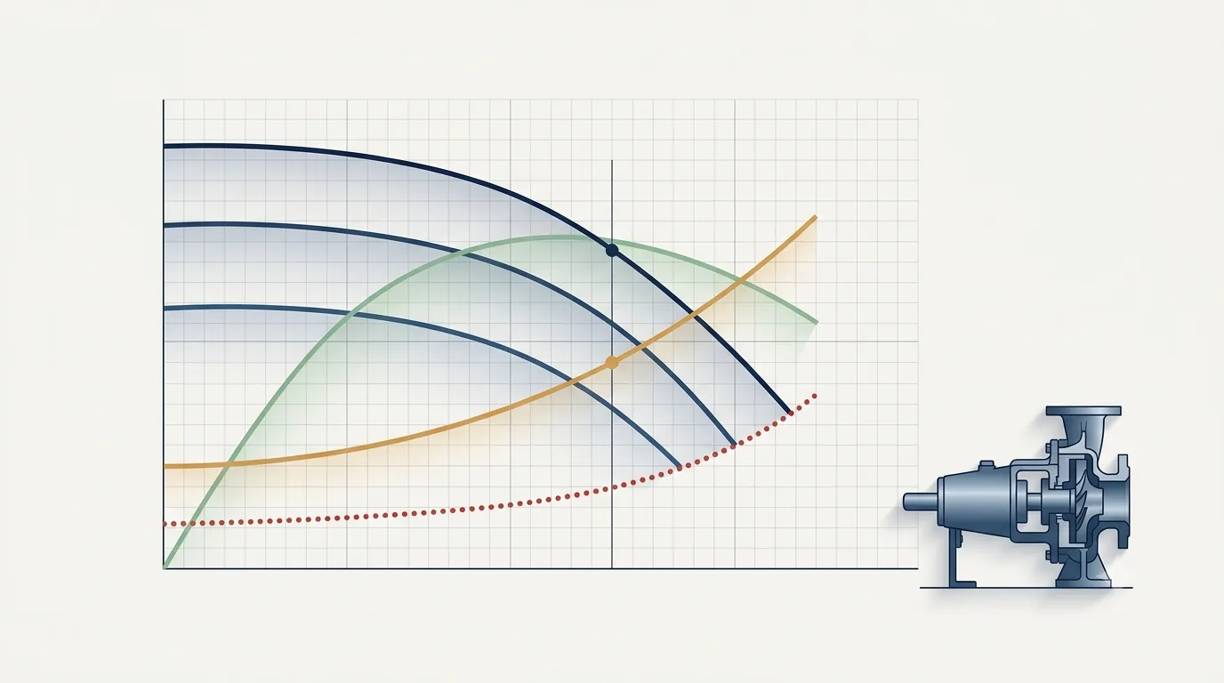
A manufacturer curve sheet is four families of information stacked on one chart — head, efficiency, power and NPSHr — and every one of them must be read at the same flow. Most field failures traced back to “the pump” are really failures to read that sheet properly.
1 · What the curve sheet actually is
The performance curve in a pump datasheet is not a drawing — it is test data. The manufacturer ran the pump (or a homologous model of it) on a test rig, measured flow, head, power and suction performance, and plotted the results per the acceptance-test standards ISO 9906 or ANSI/HI 14.6. Three consequences follow immediately, and each one changes how you read the sheet:
- It is valid for one speed, one impeller diameter, and one fluid — almost always clean cold water, SG = 1.0, at the rated speed printed in the title block. Change any of these and the curve must be corrected, not reused.
- It carries a tolerance, not a guarantee of exactness. The acceptance grade (Section 5) defines how far the delivered pump may deviate from the printed line — and ±5% head on a flat curve can move the duty flow a long way.
- The catalogue chart is usually a family, not your pump. What you see is the full-diameter and minimum-diameter envelope with intermediate trims. Your pump is one line in that family — and often an interpolated trim between two printed ones.
2 · The four families on one chart
A complete curve sheet stacks four relationships against the same flow axis. Each answers a different design question:
| Curve | Axis | Decides | Typical misreading |
|---|---|---|---|
| H–Q (one per trim) | Head, m | Whether the pump meets the duty; where it intersects the system curve | Reading the envelope or the wrong trim line |
| Efficiency η | % | Energy cost; how far the duty sits from BEP | Quoting BEP efficiency at a non-BEP duty |
| Power P2 | kW | Motor size — including at end of curve, not just at duty | Forgetting it is plotted for water, SG = 1.0 |
| NPSHr (NPSH3) | m | Suction safety, with margin — see the NPSH design guide | Treating NPSHr as “safe” instead of “already cavitating 3%” |
Two of these need a precise definition, because the names mislead:
P2 is shaft power — the mechanical power absorbed at the pump coupling, not the electrical power drawn from the wall (that is P1, larger by the motor and drive losses). It relates to the hydraulic power through the pump efficiency:
NPSHr on the sheet is NPSH3 — by definition, the suction head at which the pump has already lost 3% of its head to cavitation. It is a test criterion, not a safety boundary. A pump operating with NPSH available exactly equal to NPSHr is cavitating by definition; HI 9.6.1 margins exist precisely because of this[4].
3 · Interactive: the curve-sheet explorer
The model below is a realistic medium-size water pump at 1,480 rpm with four impeller trims (430 / 410 / 390 / 370 mm). Move the duty flow and switch trims — the vertical line is the “read everything here” discipline made visible.
Try this: hold the duty at 1,100 m³/h and trim down to 370 mm. Head and power fall — but NPSHr does not move, because trimming the outer diameter does nothing to the impeller eye. Then push the flow to 1,800 m³/h and watch NPSHr climb the steep right-hand wall while efficiency collapses.
4 · Worked example — reading one duty completely
Required duty: 1,000 m³/h at 45 m. On the family above, the full 430 mm impeller gives 52.0 m at 1,000 m³/h — too much. The 390 mm trim gives 41.4 m — too little. The 410 mm trim gives 46.5 m, slightly above the requirement: the correct selection (the surplus is absorbed as the duty point slides marginally up the system curve — never select a trim that falls short).
Now the vertical line at 1,000 m³/h on the 410 mm trim, reading all four families:
| Quantity | Value | Design consequence |
|---|---|---|
| Head H | 46.5 m | Meets the 45 m duty with a small surplus ✓ |
| Efficiency η | 84.4% | Duty sits at 94% of this trim's BEP (≈ 1,060 m³/h) — inside POR ✓ |
| Power P2 | 150 kW | At end of allowable region (120% BEP ≈ 1,272 m³/h): 175 kW |
| NPSHr (NPSH3) | 4.0 m | With HI margin ratio 1.3 → require NPSHa ≥ 5.2 m |
The motor decision shows why the power family must be read across the whole operating region, not at one point: duty power is 150 kW, and the habitual “duty + 10%” rule suggests 165 kW. But if operation can ever reach the right-hand end of the allowable region, absorbed power reaches 175 kW. The next standard IEC rating, 200 kW, covers both — and the selection is documented as non-overloading across the AOR, not as a margin guess.
5 · The curve is a band, not a line — ISO 9906 grades
Acceptance standards define how far the delivered pump may deviate from the quoted curve. Under ISO 9906:2012 (harmonised with ANSI/HI 14.6), the common grades are[1,2]:
| Grade | Flow ΔQ | Head ΔH | Efficiency Δη | Typical use |
|---|---|---|---|---|
| 1B | ±4.5% | ±3% | −3% | Large / high-energy pumps, contractual efficiency |
| 2B | ±8% | ±5% | −5% | Standard water & wastewater duty (the usual default) |
| 3B | ±9% | ±7% | −7% | Small, mass-produced pumps |
Grade 1U and 1E variants tighten this further (1U allows only positive tolerance; 1E adds a non-negative efficiency tolerance). The design consequence is rarely appreciated: on a flat pump curve, a −5% head tolerance at the duty head can shift the achieved flow by far more than 5% — exactly the geometry problem described in the system head curve article. If the process genuinely needs a minimum flow, specify the guarantee point and grade accordingly, and say so in the datasheet — “Grade 2B” silently accepted from the quotation is a decision, whether you made it or not.
6 · Speed & trim — using the affinity laws on the whole curve
Catalogue curves are printed for one speed. Run the pump on a VFD, or order a different trim, and the affinity laws scale the entire curve, point by point:
Three corrections to the way these laws are commonly used:
- They map curve to curve, not duty to duty. The laws connect homologous points — the same point on the scaled curve. Your new duty point is found by intersecting the scaled curve with the system curve; it is not the old duty point scaled.
- % speed ≠ % flow whenever static head exists. The “20% speed = 20% flow = 50% power” story is true only for purely frictional systems. With static head, flow falls faster than speed — and below the speed where the scaled shut-off head equals the static head, flow stops entirely.
- Trim is not exactly affinity. Diameter scaling \(Q\propto D,\ H\propto D^2\) is a first estimate; real trims lose some efficiency and deviate from the square law because the casing stays the same size. Use the manufacturer's tested trim curves for selection, and limit trims to roughly 75–80% of full diameter[6].
7 · Interactive: speed correction against a real system
With 20 m static, 90% speed delivers only ≈ 85% flow — and below ≈ 58% speed the pump dead-heads against the static column and delivers nothing. Set static to 0 m and the cube-law story comes back: 90% speed → 90% flow → 73% power.
8 · Viscosity — the silent curve killer
Everything so far assumed water. Pump a viscous fluid — sludge, glycerine solutions, oils, some polymers — and the water curve must be derated. The Hydraulic Institute method (ANSI/HI 9.6.7) condenses the physics into a single parameter B computed at the water BEP, from which three correction factors follow[5]:
with ν in cSt, Q in m³/h, H in m and N in rpm. The corrected performance is \(Q_{vis}=C_Q\,Q_w\), \(H_{vis}=C_H\,H_w\), \(\eta_{vis}=C_\eta\,\eta_w\) — and the pattern of the factors is the important lesson: flow and head survive moderate viscosity almost intact, but efficiency does not. At 120 cSt on the pump above, B ≈ 2.7: flow and head keep ~99% of their water values, while efficiency keeps only ~90% — and absorbed power rises accordingly (times the fluid SG, on top).
9 · Interactive: HI viscosity correction
Slide to 500 cSt: flow and head still keep ~94% — but efficiency keeps only 74% of its water value (85% → ~63% absolute) and shaft power is up ~19% before the SG multiplier. Then slide the specific gravity up and watch only the amber power curve rise: head in metres and efficiency are blind to density — the kilowatts are not. Size the motor for the viscous condition, never from the water sheet.
10 · The misreadings that cause field failures
Every one of these is a real failure pattern, and every one originates on paper, not in the machine:
- Reading the family envelope instead of the quoted trim. The catalogue page shows max-to-min trim; the delivered pump is one line. A duty read off the full-diameter curve but supplied as a 390 mm trim is short by 10 m of head before it ever starts.
- Treating the printed line as exact. A Grade 2B pump may legally deliver 5% less head. On a flat curve crossing a flat system curve, that can be a 15–20% flow shortfall — contractually acceptable, hydraulically disastrous if you never specified the grade.
- Quoting BEP efficiency at a non-BEP duty. The energy study used 85%; the pump runs at 70% of BEP where the sheet reads 78%. Every kWh estimate downstream of that number is wrong.
- Sizing the motor at the duty point. Rising power toward runout plus any future drop in system resistance equals overload trips. Read P2 at the end of the allowable operating region — and check it again for SG and viscosity if the fluid is not cold water.
- Reading NPSHr as a safety line. NPSH3 means 3% head loss already occurring. Apply the HI 9.6.1 margin (ratio ≥ 1.1–1.3 for typical water duties, more for high-energy pumps) above the curve value — at the highest expected flow, where NPSHr is steepest.
- Expecting trim to fix suction problems. Trimming reduces head and power; the impeller eye — and therefore NPSHr at a given flow — stays essentially unchanged.
- Using a 50 Hz curve for a 60 Hz pump (or vice versa). A 20% speed difference moves head by 44% and power by 73%. Always confirm the rated speed in the title block matches the site supply and motor.
- Assuming % speed = % flow on a VFD. True only with zero static head. With static head the turndown range is far narrower than the drive range — and below the no-flow speed the pump churns at shut-off, which is a reliability event, not a control state (see the VFD myth).
- Ignoring the limits the sheet does not print. Minimum continuous stable flow (often 40–70% of BEP depending on the pump), maximum casing pressure, and allowable operating region boundaries frequently live in the selection software or the O&M manual — ask for them and put them on the datasheet.
11 · Curve-reading checklist
- Confirm the title block first: speed, impeller diameter, fluid, temperature, test standard and acceptance grade — before reading a single value.
- One vertical line: read H, η, P2 and NPSHr at the same flow, on the same trim.
- Locate the duty relative to BEP and confirm it sits inside the POR (70–120% of BEP per HI 9.6.3) for every expected operating mode — not just the design point.
- Read power at the end of the allowable region, correct for SG and viscosity, then size the motor as non-overloading.
- Add the NPSH margin to the curve value at the highest expected flow, per HI 9.6.1.
- Scale curves, not points, when applying affinity for speed — and use tested trim curves rather than the square law where they exist.
- Specify the acceptance grade in the procurement documents if the duty actually matters; demand the witnessed test for large machines.
- Ask for what is not printed: MCSF, allowable region limits, maximum working pressure, and the tested — not interpolated — curve for the exact trim supplied.
References & standards
- ISO 9906:2012. Rotodynamic pumps — Hydraulic performance acceptance tests — Grades 1, 2 and 3.
- Hydraulic Institute. ANSI/HI 14.6 — Rotodynamic Pumps for Hydraulic Performance Acceptance Tests.
- Hydraulic Institute. ANSI/HI 9.6.3 — Rotodynamic Pumps: Guideline for Operating Regions (POR / AOR).
- Hydraulic Institute. ANSI/HI 9.6.1 — Rotodynamic Pumps: Guideline for NPSH Margin.
- Hydraulic Institute. ANSI/HI 9.6.7 — Rotodynamic Pumps: Guideline for Effects of Liquid Viscosity on Performance.
- Gülich, J.F. Centrifugal Pumps, 4th ed. Springer, 2020 (trim deviations, curve shapes, suction behaviour).
- Karassik, I.J., Messina, J.P., Cooper, P., Heald, C.C. Pump Handbook, 4th ed. McGraw-Hill, 2008.
- Jones, G.M. (ed.). Pumping Station Design, 3rd ed. Butterworth-Heinemann, 2008.
- Flowserve / Cameron. Cameron Hydraulic Data Book, 19th ed. (curve reading and corrections).
- U.S. DOE & Hydraulic Institute. Improving Pumping System Performance: A Sourcebook for Industry, 2nd ed.