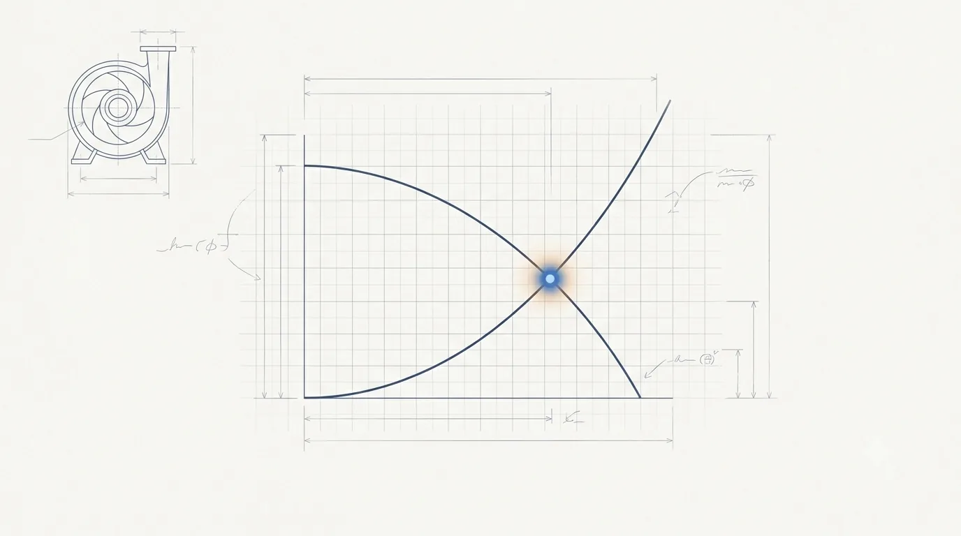
Why the pump you select never operates where the catalogue says it will — and how to make the system, not the salesman, decide the duty point.
1 · Anatomy of the system head curve
A centrifugal pump does not have a flow rate. It has a capability — its head–capacity (H–Q) curve — and the flow it actually delivers is dictated entirely by the resistance of the system connected to it. That resistance, plotted against flow, is the system head curve, and the single point where it crosses the pump curve is the only flow and head the machine can physically produce.
Every system head curve is the sum of two physically distinct components:
1. Static head — the elevation and pressure the pump must overcome regardless of flow. It is the height water must be lifted from the supply liquid level to the discharge level, plus any difference in surface pressure. On a curve it is a horizontal line: it exists even at zero flow.
2. Dynamic (friction) head — the energy dissipated moving the liquid through pipe, fittings, valves and equipment. It is zero at zero flow and rises steeply — very nearly with the square of flow. This term bends the curve upward into the familiar parabola.
2 · Building the system curve
The friction component is computed from a head-loss equation evaluated across the full flow range. Two formulations dominate water practice.
Darcy–Weisbach (universal, physically rigorous)
Valid for any fluid and flow regime, it expresses loss in terms of the friction factor \(f\):
Substituting \(V = 4Q/\pi D^2\) collapses the loss into a clean \(Q^2\) relationship. Minor losses from bends, valves and transitions add as \( \sum K \cdot V^2/2g\), which is also proportional to \(Q^2\). Everything that varies with velocity therefore lumps into a single system resistance coefficient \(K\):
Hazen–Williams (water-specific, code-friendly)
Widely embedded in water-utility design and the basis of most pipeline specifications, it uses an empirical roughness coefficient \(C\):
The shape of the curve tells you the system type
| System type | Static : friction | Curve shape | Design implication |
|---|---|---|---|
| High-static (transmission lift, reservoir filling) | High static, low friction | Nearly flat, high intercept | VFD savings limited; affinity laws misleading |
| Balanced (typical pump stations) | Comparable | Moderate parabola | Standard selection; modest VFD benefit |
| High-friction (closed loops, long small-bore mains) | Low static, high friction | Steep parabola from near origin | VFD highly effective; cube-law savings approached |
3 · The pump curve & the operating point
The manufacturer supplies the pump H–Q curve: head falling as flow rises, for a given impeller diameter and speed. Superimpose it on the system curve and they intersect at exactly one flow. That intersection is the operating point (or duty point) — the steady-state equilibrium where the head the pump generates equals the head the system demands.
Approximating both curves as parabolas makes the equilibrium explicit. With a pump curve \(H_p = H_0 - c\,Q^2\) and a system curve \(H_{sys} = H_{static} + d\,Q^2\), setting them equal gives the operating flow in closed form:
Two consequences follow immediately, and both are routinely violated on real projects:
- Raise the static head (a fuller reservoir, a higher discharge) and the operating point slides up and to the left — less flow, more head. A pump sized for an empty reservoir is the wrong pump for a full one.
- Add friction (a throttled valve, a fouled pipe, an undersized main) and the system curve steepens, again pushing the duty point left. Throttling does not change the pump; it changes the system the pump sees.
The interactive figure below lets you move both and watch the duty point respond in real time.
4 · Interactive: matching pump to system
Notice that throttling (raising friction) and trimming both move the duty flow toward BEP — but only one of them does it without burning the energy as heat across a valve. Section 8 returns to this.
5 · Worked example — transmission pump station
A station lifts treated water from a clearwell to an elevated balancing reservoir through a ductile-iron transmission main. The design parameters:
| Parameter | Value | Note |
|---|---|---|
| Design flow, \(Q_d\) | 1,080 m³/h (0.30 m³/s) | Single duty pump |
| Static lift, \(H_{static}\) | 45.0 m | Clearwell LWL to reservoir TWL |
| Pipe: DI, cement-lined | DN 500, L = 2,000 m | Hazen–Williams C = 130 |
| Velocity at \(Q_d\) | 1.53 m/s | Within 1–2 m/s economic band |
| Friction loss, \(h_f\) | 8.2 m | Hazen–Williams + minor losses |
| Required duty head | 53.2 m | \(45.0 + 8.2\) |
The system resistance coefficient back-calculates from the design point:
A pump with a shut-off head \(H_0 = 68\ \text{m}\) and curve \(H_p = 68 - 1.27\times10^{-5}\,Q^2\) is selected. Solving for the intersection:
The pump's BEP sits at 1,152 m³/h (η ≈ 84%), so the duty point is at 94% of BEP — comfortably inside the preferred operating region. The absorbed shaft power:
6 · BEP, POR & AOR — where you are allowed to operate
The Best Efficiency Point is not merely the peak of the efficiency curve. It is the flow at which the liquid enters the impeller with minimum incidence, internal recirculation is suppressed, and hydraulic radial and axial loads on the shaft are at their minimum. Drift away from BEP and reliability — not just energy cost — degrades.
The Hydraulic Institute codifies two windows around BEP [1]:
| Region | Typical range | What happens here |
|---|---|---|
| POR — Preferred Operating Region | ~70% – 120% of BEP | Vibration and loads low; the target band for continuous duty |
| AOR — Allowable Operating Region | Manufacturer-defined, wider | Acceptable but with reduced service life / higher vibration limits |
| Below AOR (low flow) | < ~40–50% BEP | Suction & discharge recirculation, temperature rise, cavitation, shaft deflection |
| Above AOR (runout) | > ~120–130% BEP | NPSH-limited cavitation, motor overload, steep efficiency fall-off |
7 · The oversizing trap
The most common — and most expensive — selection error in the industry is conservative margin stacking. A process engineer adds 10% to the flow "to be safe", the hydraulic engineer adds another head margin for "future fouling", a third margin covers pipe ageing. Each is individually defensible; compounded, they select a pump whose curve sits well above the true system curve.
The pump then does one of two things, both bad:
- It overpumps. Against the actual system the duty point lands far to the right — more flow than needed, higher velocity, elevated NPSH demand, motor pushed toward overload.
- It gets throttled back. To force design flow, a control valve is closed, adding artificial friction. The duty point moves left of BEP, efficiency collapses, and the throttled energy is dissipated as heat and noise across the valve.
The figure below contrasts a correctly matched pump with an oversized one throttled to deliver the same design flow.
| Metric | Matched pump | Oversized + throttled |
|---|---|---|
| Shut-off head | 68 m | 82 m |
| Head actually required by system | 53 m | 53 m |
| Head produced (before valve) | 53 m | 66 m |
| Head burned across throttle valve | 0 m | ~13 m |
| Operating efficiency | ~84% | ~75% |
| Approx. shaft power | 186 kW | ~259 kW |
| % of BEP | 94% | ~78% (and falling) |
8 · Controlling the operating point
When the duty point needs to move — because demand varies, or because the selected pump is slightly off — there are three levers, in ascending order of merit:
| Method | Mechanism | Verdict |
|---|---|---|
| Throttling | Adds friction; steepens system curve | Simplest, worst. Energy destroyed across the valve permanently |
| Impeller trim | Permanently scales the pump curve down: \(H \propto (D'/D)^2\) | Cheap, permanent, efficient — ideal when the duty is fixed and slightly high |
| Variable speed (VFD) | Scales the whole curve with speed | Best for variable demand; savings depend heavily on the static/friction split |
All three are governed by the affinity laws, which relate a rotodynamic pump's performance to speed \(N\) (or trimmed diameter):
9 · Design checklist & engineering judgement
- Build the system curve before opening any catalogue. Separate static and friction explicitly; never let a vendor hand you both the system and the pump.
- Bracket the static head. Compute duty points at minimum and maximum reservoir/tank levels — the pump must behave at both extremes, not just the design average.
- Plot the curve family. Clean vs. fouled (aged \(C\)), single vs. parallel operation, and the future-flow case. The duty point lives somewhere in that envelope, not on a single line.
- Land the design point at 100–110% of BEP flow when growth is expected, so the pump migrates toward BEP over its life rather than away from it.
- Resist margin stacking. Apply one rational, documented margin — not three hidden ones. Prefer a trimmable impeller or a VFD over throttling away a fat selection.
- Verify the suction side independently. A perfect duty point is worthless if NPSHa < NPSHr there.
References & standards
- Hydraulic Institute (HI). ANSI/HI 9.6.3 — Rotodynamic Pumps: Guideline for Operating Regions. Parsippany, NJ.
- Hydraulic Institute (HI). ANSI/HI 9.6.1 — Rotodynamic Pumps: Guideline for NPSH Margin.
- Hydraulic Institute (HI). ANSI/HI 14.3 — Rotodynamic Pumps for Design and Application.
- Karassik, I.J., Messina, J.P., Cooper, P., Heald, C.C. Pump Handbook, 4th ed. McGraw-Hill, 2008.
- Europump & Hydraulic Institute. Pump Life Cycle Costs: A Guide to LCC Analysis for Pumping Systems.
- Gülich, J.F. Centrifugal Pumps, 4th ed. Springer, 2020.
- U.S. DOE / HI. Improving Pumping System Performance: A Sourcebook for Industry, 2nd ed.
- AWWA Manual M11, Steel Pipe — A Guide for Design and Installation (head-loss methods & Hazen–Williams C values).
- Crane Co. Technical Paper No. 410 (TP-410) — Flow of Fluids Through Valves, Fittings, and Pipe.