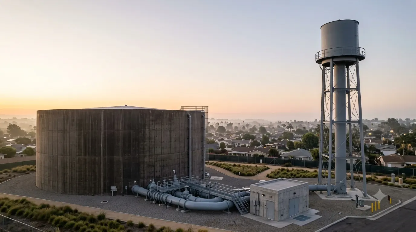
A water source delivers at the rate that is cheapest to build and run — steady, around the clock. A city drinks in pulses: almost nothing at 4 a.m., a wall of demand at 7. Storage is the buffer that absorbs the difference. Get its volume wrong in one direction and taps run dry at the morning peak; wrong in the other, and the water sits so long the chlorine dies before it reaches the house. This is the engineering of that single number.
1 · Why store water at all
The instinct that "more storage is safer" is the most expensive instinct in distribution design. Storage exists to decouple supply from demand — to let the production side (the treatment plant, the well field, the transmission main) run at a flat, efficient, capital-minimal rate while the consumption side does whatever 200,000 people decide to do with their taps. A reservoir buys four distinct things at once:
- It flattens the production rate. Without storage, the plant and the transmission main must be sized for the peak hour. With storage, they are sized for the maximum day — a far smaller, cheaper number. The tank pays for the pipe it lets you not build.
- It holds pressure. An elevated reservoir or a ground tank feeding a booster sets the hydraulic grade line; it stabilises pressure across the network as demand swings, and rides through pump stop/start transients (see reservoir vs. tank boundary conditions).
- It survives failure. When a pump trips, a main breaks, or the power fails, storage is the only thing standing between the city and a dry network — the minutes-to-hours of grace in which the system is repaired.
- It fights fire. The single largest instantaneous draw a network ever sees is not a person — it is a fire hydrant. Storage holds that volume so the distribution mains do not have to carry it.
2 · The three volumes inside every reservoir
Strip away the pressure-holding role (which is about elevation, not volume) and a storage reservoir holds three stacked volumes. Every credible design standard — the Ten States Standards[1], AWWA M31[2] and M32[3] — partitions storage this way:
| Component | Sized by | Insures against |
|---|---|---|
| Balancing (operational / equalizing) | The daily demand curve vs. the supply rate | The predictable diurnal peak — every single day |
| Fire | Needed fire flow × duration (code / risk) | The largest credible single fire |
| Emergency | Credible outage duration × demand | Pump trip, main break, power loss |
Two of these scale with the population; one does not. Balancing and emergency storage grow with demand. Fire storage is set by the worst building, not the headcount — a town of 5,000 with a hospital can need more fire storage than a bedroom suburb of 50,000. That single asymmetry, which we will see in the second chart, governs the shape of small-system storage.
3 · From population to the numbers that size a tank
Everything starts with three demand figures derived from the population \(P\) and the per-capita demand \(q\):
where ADD is the average-day demand, MDD the maximum-day demand (the busiest day of the year, \(f_d\approx1.4\text{–}1.8\)), and PHD the peak-hour demand rate (\(f_h\approx2.0\text{–}3.0\) relative to the average hour). The production system is built for MDD; storage absorbs the gap between MDD-rate supply and PHD-rate demand. A worked anchor we will carry through the article:
| Quantity | Value | Rate |
|---|---|---|
| Average-day demand (ADD) | 12,500 m³/d | 521 m³/h |
| Maximum-day demand (MDD), fd=1.5 | 18,750 m³/d | 781 m³/h |
| Peak-hour demand (PHD), fh=2.5 | — | 1,302 m³/h |
4 · Balancing storage — the mass-curve method
This is the volume you can compute from first principles, and the one engineers most often guess instead. On the maximum day, the source supplies a near-constant flow; consumption follows the diurnal curve. Whenever supply exceeds demand (at night) the tank fills; whenever demand exceeds supply (morning and evening peaks) the tank drains. The required balancing volume is the full travel between the fullest and emptiest the tank gets — the peak-to-trough range of the cumulative net inflow. This is the classic Rippl mass-curve[4]:
Two design levers move this number hard. The first is the shape of the demand curve: a peakier city (a hot climate, strong evening culture) needs more balancing volume. The second — the one designers control — is the pumping window: a source that pumps 24 hours a day needs the least storage; one that pumps only 14 hours (to dodge peak electricity tariffs, or because the well can't run continuously) front-loads all its inflow into part of the day and forces the tank to carry the rest. Off-peak pumping is real money saved on the energy bill (life-cycle cost) — paid for in concrete.
5 · Interactive: the diurnal balance
The blue curve is the city drinking through the day; the amber line is the source supplying it. Where blue is below amber, the tank fills; where blue rises above amber, the tank drains. The balancing volume is the total swing between those phases.
On the defaults — 24-hour pumping, a moderate peak factor — balancing storage lands near 18% of the maximum day, squarely inside the 15–25% range the textbooks quote. Now drag the pumping window down to 14 hours: the same city suddenly needs well over 30% of MDD in concrete, because the source is silent for ten hours the tank must cover alone. That trade — kilowatt-hours against cubic metres — is the central economic decision in balancing storage.
6 · Fire storage — the volume you hope never to move
Fire storage is sized by a flow the network may never see, held for a duration it hopes never to need:
The needed fire flow \(Q_{fire}\) is not an engineering free choice — it comes from the fire code and the insurance schedule (ISO in North America; local civil-defence requirements in the Gulf), driven by the largest building's construction, area and occupancy[2,5]. A residential district might need 2,000–4,000 L/min; a hospital, mall or industrial unit can demand 8,000–16,000 L/min. The duration \(t_{fire}\) scales with that flow, typically 2 hours for modest demands rising to 4 hours for the largest.
For our town, take a governing requirement of 8,000 L/min (480 m³/h) for 3 hours:
7 · Emergency storage — sizing for the day supply fails
Emergency storage answers a risk question, not a hydraulics one: how long must the network survive with no inflow at all? A trip that auto-restarts is minutes; a ruptured transmission main with no parallel feed can be a day. The volume is the credible outage duration carried at the demand prevailing during it:
The right \(t_{out}\) is a deliberate engineering and economic judgement — set by source redundancy, the presence of a second feed, repair-crew response time, and how much risk the utility will hold. A single-source system with an 8-hour credible outage:
This is the component most sensitive to system architecture, not tank design: build a second independent transmission feed and the credible outage — and the storage it demands — collapses. Storage and redundancy are substitute goods; the cheapest resilience is usually a mix of both, decided together (see infrastructure at scale).
8 · Interactive: the total-storage stack
Now assemble all three across the full range of community sizes. Watch what happens at the small end: fire storage — flat, code-driven, indifferent to population — towers over everything. At the large end, demand-driven balancing and emergency storage take over and fire becomes a rounding error.
Slide the population down to 5,000: fire storage — unchanged at 1,440 m³ — becomes the tallest band by far, and the per-capita storage figure roughly triples. This is why small communities carry so much "spare" water per head, and why fire flow, not demand, writes the cheque for rural storage. Slide it up to 200,000 and fire all but vanishes beneath the demand stack.
9 · The hidden cost of storage — water age
Here is the tension that makes storage a genuine optimisation rather than a "bigger is safer" exercise. Every cubic metre of storage is a cubic metre of residence time. The turnover time — roughly the tank volume divided by the throughput — is how long water sits between treatment and tap:
Chlorine residual decays approximately first-order with time, at a bulk rate \(k\) that climbs with temperature — brutally relevant in the Gulf. Oversize the reservoir "to be safe" and you stretch \(\tau\); stretch \(\tau\) and the disinfectant residual collapses, nitrification and taste-and-odour problems set in, and trihalomethanes keep forming in the dark[6,7,8]. WHO and most utilities hold a residual of at least 0.2 mg/L at the far tap[9]; an over-built tank quietly spends that margin.
10 · Interactive: turnover & residual
Set how many days of supply you store, and watch the chlorine that survives to the tap. The curve is first-order decay; the marker is your turnover time; the red zone is below the 0.2 mg/L floor.
Start at the lean 0.7-day design and the residual holds comfortably. Now do what nervous committees do — drag storage to 3 days "for resilience" — and watch the residual fall through the floor, especially once you nudge \(k\) up to a summer value. That is the cost of over-sizing made visible: not money, but the disinfectant that was supposed to reach the last house.
11 · Sizing checklist for the design desk
- Build the demand basis first — ADD, MDD and PHD from population and a defensible per-capita figure; storage is downstream of these three numbers.
- Size balancing from the mass curve, on the maximum-day pattern, at the actual pumping window — not a 15–25% rule of thumb pulled from a textbook for a different city.
- Carry fire storage as a separate, dedicated line — needed fire flow × duration from the code, set by the worst building, never assumed to be "covered" by the daily swing.
- Decide emergency storage with the redundancy decision — a second feed and more storage are substitute resilience; price them together, not in separate meetings.
- Sum, then test turnover — compute τ = V/ADD and the resulting residual. If the resilient volume fails the water-age check, the answer is mixing and operating bands, not a bigger or smaller tank chosen by feel.
- Design the inlet/outlet for circulation — opposed nozzles, fill-and-draw operating bands, no short-circuit path. Volume without turnover is a liability, not a reserve.
- Re-run at the design horizon — storage sized for today's population is under-built for year 20 and over-aged for year 1; state the year it is sized for.
References & standards
- Great Lakes–Upper Mississippi River Board (GLUMRB). Recommended Standards for Water Works (Ten States Standards) — finished-water storage requirements.
- American Water Works Association. Manual M31 — Distribution System Requirements for Fire Protection.
- American Water Works Association. Manual M32 — Computer Modeling of Water Distribution Systems.
- Rippl, W. The Capacity of Storage Reservoirs for Water Supply, Proc. ICE, 1883 — the mass-curve method.
- Insurance Services Office (ISO). Guide for Determination of Needed Fire Flow; see also NFPA 22 — Water Tanks for Private Fire Protection.
- U.S. EPA. Effects of Water Age on Distribution System Water Quality. Office of Water, 2002.
- Walski, T.M., Chase, D.V., Savic, D.A. et al. Advanced Water Distribution Modeling and Management. Haestad/Bentley Press.
- American Water Works Association. Manual M42 — Steel Water-Storage Tanks; AWWA G200 — Distribution Systems Operation and Management.
- World Health Organization. Guidelines for Drinking-water Quality, 4th ed. — disinfectant residual at the point of use.