District Cooling & Energy Transfer Stations for Megatall Buildings: Delta-T, Approach & Metering

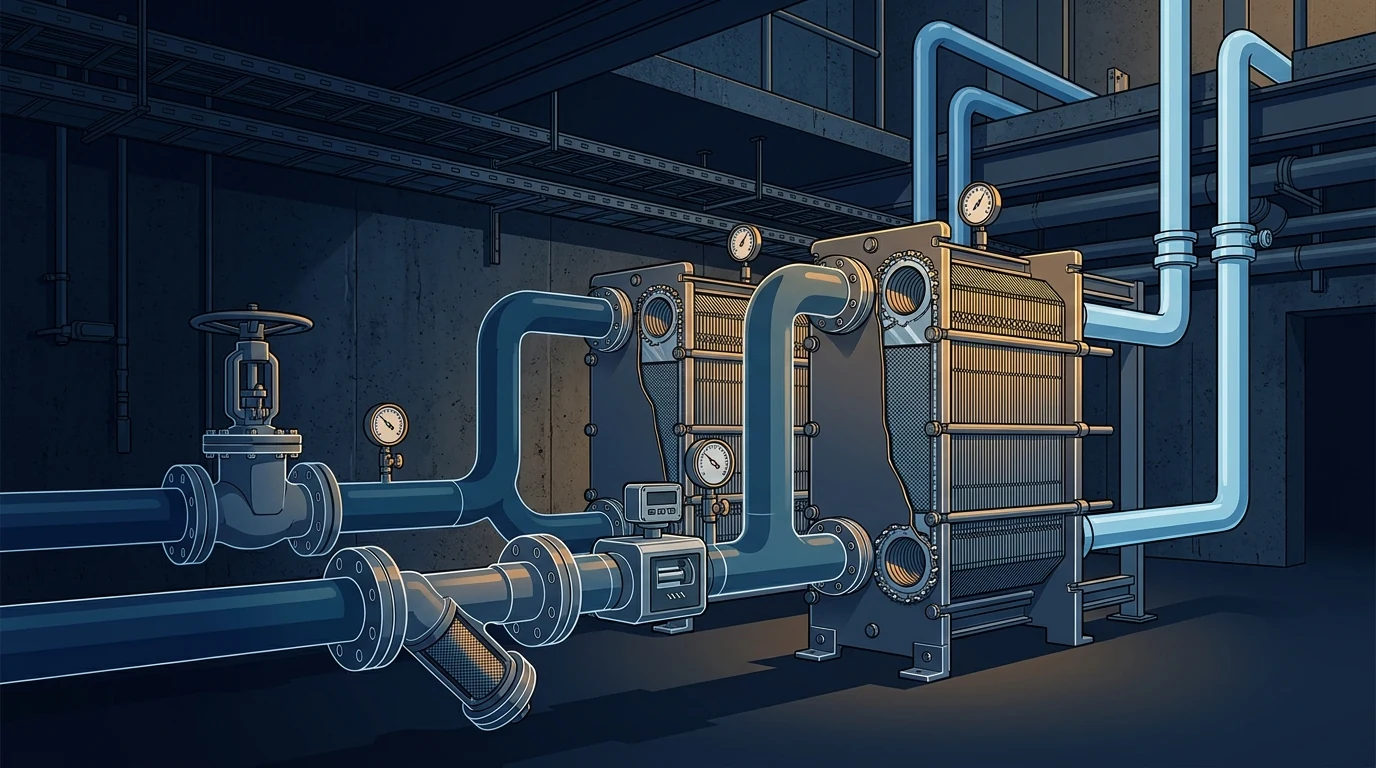
Connect a megatall tower to a district cooling network and you have not simplified the design — you have replaced a plant you control with a contract you cannot renegotiate. The provider guarantees a supply temperature and a pressure; you guarantee a return temperature. That last clause is where the money is. Every kelvin of return temperature you fail to deliver inflates the flow you must contract for, and the capacity charge follows the flow: a design ΔT of 8 K delivered as 4 K doubles the capacity charge for exactly the same cooling. The energy transfer station is a small room with four pieces of equipment in it, and it is one of the highest-leverage designs in the building.

1 · What the connection really changes

• ΔT stops being an efficiency question and becomes a bill. In an in-house plant a low ΔT wastes pump energy and forces extra chillers on — bad, but internal. On a district connection it is a contractual quantity that is metered, charged and penalised.
• You inherit somebody else's pressure. District networks run at high pressure to reach distant customers. That network pressure lands at your ETS and adds to whatever static your own building generates.
• The interface is almost always indirect. A plate heat exchanger separates the network hydraulically from the building — mandatory in a tall building, because the network cannot be exposed to a 60 bar building static and the building cannot be exposed to network transients.
• And that heat exchanger costs you temperature. The approach is added to the supply temperature the provider delivers, and the building's coils must be selected for the warmer number.
• The meter is the cash register. A BTU meter measures flow and two temperatures; at low ΔT the temperature sensors dominate the uncertainty, and the uncertainty is money.

2 · Interactive: what a degraded ΔT costs

District tariffs are typically split into a capacity charge — based on contracted peak capacity or peak flow — and a consumption charge on metered energy. Cooling delivered is unchanged by a poor ΔT; the flow to deliver it is not.

Design at 8 K and deliver 6 K and the contracted flow rises by 33 %; deliver 4 K and it doubles. On a modest 4 M annual capacity charge that is 1.33 M a year for nothing — no extra cooling, no extra comfort, just warmer water going back. The causes are all inside your boundary and all fixable at design: three-port valves anywhere in the building, open bypasses, coils selected at a narrower ΔT than the contract, decoupler backflow, and control valves with too little authority to close properly. This is the single strongest reason to design a district-connected tower at a wide ΔT and then defend it — the same argument as in chilled-water pumps, but with an invoice attached.

3 · The energy transfer station

An indirect ETS is deceptively simple: a plate heat exchanger, a control valve on the primary, isolation and strainers, and a meter. Each of those four is a common failure point:

• The heat exchanger. Sized on approach, fouling allowance and both-side pressure drops, and rated for the primary network pressure on one side and the building static on the other. Specify the plate material and gasket for the network's water chemistry, and provide space to open the plate pack — an exchanger that cannot be stripped will not be cleaned.
• The primary control valve. This is the component that actually delivers your ΔT. It must have real authority against the network's differential pressure — which is large and varies with the network's own load — so it is almost always a pressure-independent control valve. An ordinary two-port valve on a district primary is the classic cause of a building that cannot hold its return temperature.
• Strainers and filtration. The network is a shared system carrying everybody's debris. Provide a properly sized primary strainer with differential-pressure monitoring, and consider side-stream filtration; a fouled plate pack shows up first as a widening approach and then as a ΔT failure.
• The meter. Located, installed and maintained to the standard the contract references — with the straight lengths the flow meter actually needs and the matched sensor pair in the correct pockets.

4 · Interactive: the approach you pay for twice

The heat exchanger's approach adds to the supply temperature the building sees, and a warmer supply means every coil in the tower must be larger to do the same job — because coil capacity follows the log-mean temperature difference, which shrinks fast as the supply warms.

With a 4.5 °C primary and a 1.5 K approach the building gets 6.0 °C — exactly the reference selection, so the coils are unchanged. Loosen the approach to 3 K to save money on plates and the secondary rises to 7.5 °C, the LMTD shrinks from 8.4 K to 6.9 K, and every coil in the tower needs roughly 22 % more area to deliver the same duty. That is the approach paid for twice: once in the exchanger you did not buy, and again in a thousand coils and the fan energy to push air through them. Buy the plates.

5 · Interactive: the meter is the cash register

A BTU meter computes energy from a flow measurement and a temperature difference. Because the difference is small, the temperature sensors contribute far more uncertainty than their absolute accuracy suggests — and the smaller your ΔT, the worse it gets.

At a 6 K operating ΔT with a decent 0.1 K matched sensor pair, the metering uncertainty is about 2.8 % — on a 10 M invoice, 0.28 M a year of pure measurement uncertainty. Let the ΔT fall to 4 K and it rises to 3.8 %; use ordinary 0.2 K sensors instead of a matched pair and it roughly doubles again. Two conclusions follow, and both are cheap at design stage: specify a matched sensor pair to the standard the contract cites and install them in the correct pockets, and remember that protecting ΔT improves the accuracy of your own bill as well as its size. A meter is not a commodity item on a district connection; it is the instrument that decides what you pay for twenty years.

6 · Pressure, transients and the interface

• Rate the primary side for the network, not the building. District networks run at high pressure and are subject to transients from pumping stations kilometres away. Get the network's maximum operating and test pressures in writing and rate the primary side, the exchanger and the meter accordingly.
• Rate the secondary side for the building's own static. In a tall tower the ETS often sits at the bottom, where the building-side static is highest — see the zoning discussion in chilled-water pumps.
• Protect against transients. A large primary control valve closing quickly against a long network main is a water-hammer source; specify closure times and check them, and coordinate with the network operator.
• Provide isolation that lets you work. Double isolation and a drain on the primary, so the ETS can be serviced without the network operator attending, and a bypass arrangement if the contract allows it.
• Agree the boundary in writing. Who owns the meter, who owns the strainer, who may operate the primary valves, and what the response time is when the network fails — these are design-stage decisions that end up in the O&M and in disputes.

7 · Installation & execution tricks

• Give the flow meter its straight lengths. The commonest metering error on site is an elbow immediately upstream. Reserve the upstream and downstream straight runs on the drawing and defend them in coordination — they are usually 10D and 5D but check the meter's own requirement.
• Install the sensor pair in the specified pockets, fully immersed, with the pockets in the correct locations relative to the exchanger and the meter, and keep the pair together — a matched pair separated during installation is no longer matched.
• Flush before the exchanger is connected. Commission the building side to a stated cleanliness standard with temporary spool pieces in place of the plate pack; a new plate pack fouled by construction debris starts life with a widened approach it never recovers from.
• Record the approach at commissioning and trend it. A rising approach is the single best early indicator of fouling, and it will move before anyone notices a ΔT problem.
• Commission the ΔT, not just the flow. Verify the return temperature at the ETS across the load range, and trend it against the contract from day one — the first year's data is what you will need if the ΔT clause is ever disputed.
• Alarm on ΔT. A BMS alarm on sustained low return temperature turns a slow financial leak into an actionable event. It is one line of logic and it is almost never there.
• Keep the plate pack accessible and record the tightened dimension of the pack; over-tightening a gasketed exchanger to stop a leak is how plates get crushed.

8 · The design & installation checklist

• Design at a wide ΔT and defend it — two-port valves, no bypasses, coils selected for the contract ΔT, valve authority checked.
• Use pressure-independent control valves on the primary and at the terminals.
• Buy the closer approach — it is cheaper than the coil area and fan energy it saves.
• Rate each side for its own pressure regime, with the network's figures obtained in writing.
• Specify a matched sensor pair and a properly installed flow meter, to the standard the contract cites.
• Reserve the meter's straight lengths on the drawing.
• Provide strainers with DP monitoring and consider side-stream filtration.
• Trend approach and ΔT from handover, with a BMS alarm on sustained low return temperature.
• Write the operational boundary down — ownership, access, isolation and failure response.

References & standards

1. ASHRAE District Cooling Guide, 2nd ed. — network design, energy transfer stations, ΔT management and customer interface.
2. International District Energy Association (IDEA) — district cooling best practice, contracting models and delta-T requirements.
3. EN 1434 / OIML R75 — heat and cooling meters: accuracy classes, matched temperature sensor pairs and installation requirements.
4. Taylor, S.T. Degrading Chilled Water Plant Delta-T: Causes and Mitigation, ASHRAE Transactions — the mechanisms behind low-ΔT syndrome.
5. ASHRAE Handbook — HVAC Systems and Equipment, District Heating and Cooling chapter; and the Heat Exchangers chapter for plate exchanger selection and fouling.
6. Saudi Building Code SBC 501 and the Saudi regulatory framework for district cooling services and metering.
7. CIBSE CP1 Heat Networks: Code of Practice and CIBSE Guide B — substation design, metering and commissioning practice transferable to cooling networks.
8. ASHRAE Design Guide for Tall, Supertall, and Megatall Building Systems, 2nd ed. — pressure zoning of the building side and interface location in tall buildings.