Introduction
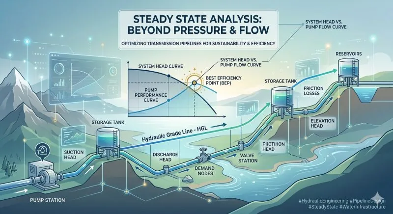
Before any transient or surge analysis can be meaningful, the steady state hydraulic model must be correct. Steady state analysis examines how a water transmission system behaves when inputs and outputs remain constant over time — establishing the baseline from which all transient events are measured.
1. Three Core Pillars of Steady State Analysis
Pillar 1: Friction Losses
Using Hazen-Williams or Darcy-Weisbach equations to determine optimal pipe diameter, the engineer is balancing capital expenditure against long-term energy costs:
- Smaller diameter → lower pipe cost, higher friction, higher energy consumption
- Larger diameter → higher pipe cost, lower friction, lower energy cost over 25–50 year life
- Optimal diameter minimises the sum of these competing costs over the project life
Pillar 2: System Head vs. Pump Curve Intersection
The operating point where the system curve intersects the pump curve is the system's "heartbeat." Good design ensures pumps operate near their Best Efficiency Point (BEP) under normal conditions. A mismatch here causes:
- Operation far from BEP, increasing vibration and energy waste
- Potential for pump surging or cavitation at extreme operating points
Pillar 3: Pressure Management
Verifying that minimum pressure requirements are met at all demand nodes while preventing excessive pressure at low-elevation points. Large transmission systems often require pressure reducing stations at intermediate points to prevent over-pressurization downstream.
2. Why Steady State Must Come First
- Energy Optimisation: Identifies oversized pipes or under-sized pumps before construction
- System Stability: Validates system behavior under varying operational scenarios
- Future-Proofing: Simulates demand growth to ensure infrastructure remains adequate for design horizon
- Transient Baseline: Provides the initial conditions from which all transient events are simulated