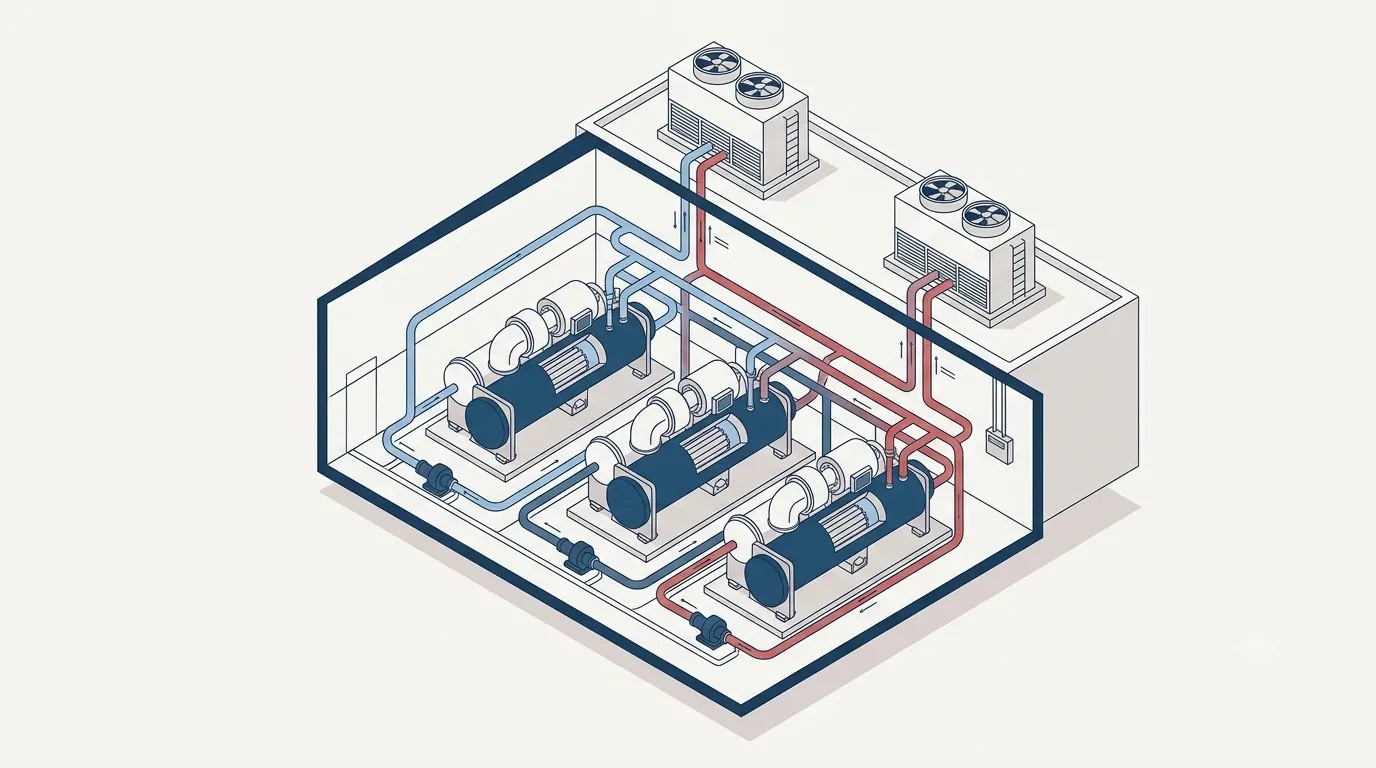
A chiller plant is the single largest energy consumer in most large buildings, and it is where the widest gap opens between the design on paper and the plant that actually runs. The chillers themselves are reliable, well-engineered machines; what goes wrong is everything around them — how they are configured, how they are staged, the water temperatures they are fed, and how they were piped and commissioned. This is a tour of the whole plant: the configurations you can choose, the design pitfalls that quietly waste energy for twenty years, and the installation problems that show up on day one.
1 · The plant is a system, not a chiller
A central chilled-water plant is a loop of loops. Chillers make cold water; primary (evaporator) pumps push it through the chillers; secondary (distribution) pumps send it up the building to the air-handling coils; and on the hot side, condenser pumps and cooling towers reject the heat to atmosphere. Get any one of those wrong and the chillers — however good — cannot deliver. This article is the plant-level companion to the source-to-terminal walk-through in the HVAC module of the MEP course; here we go deep on the plant room itself.
2 · Chiller types — the first fork
Before configuration comes selection. The dominant machines are vapour-compression chillers, split first by how they reject heat and then by compressor type[1]:
| Type | Where it fits | Efficiency & notes |
|---|---|---|
| Air-cooled | Small–medium loads, no water available, simpler O&M | Lower efficiency (rejects to dry-bulb air); no cooling tower or condenser water |
| Water-cooled | Large plants, district cooling | Best efficiency (rejects to wet-bulb); needs towers, condenser pumps & water treatment |
| Scroll / screw (positive-displacement) | Small–mid capacity, good at part load | Robust, modular; screw common 200–800 TR |
| Centrifugal | Large capacity (500 TR–several thousand) | Highest full-load efficiency; VSD centrifugals excel at part load |
| Absorption | Where waste heat / cheap gas exists | Thermally driven, low electrical use, lower COP; niche |
For a large building or a campus, the answer is almost always multiple water-cooled centrifugal (often VSD) chillers, and the rest of this article assumes that plant. The number and size of those units is the first real design decision — and the subject of the first chart.
3 · Plant configurations — how the loops are arranged
The same chillers can be piped in fundamentally different ways, and the choice sets the plant's efficiency ceiling for its whole life[2][3]:
- Constant primary flow. One set of pumps, constant flow through chillers and out to the building; capacity is trimmed by three-way valves that bypass water around the coils. Simple, cheap, and energy-hungry — flow never falls, so pumping is flat at full power all year. Obsolete for anything large.
- Primary–secondary (decoupled). Constant flow through the chillers (primary), variable flow to the building (secondary VFD pumps), separated by a short decoupler. For decades the standard: it protects each chiller's minimum evaporator flow while letting distribution flow track load. Its weakness is the decoupler, where the Low Delta-T Syndrome does its damage.
- Variable primary flow (VPF). A single set of variable-speed pumps modulates flow through the chillers themselves, down to each chiller's minimum, with a small bypass valve for the low-flow limit. Fewer pumps, lower first cost and the best pumping energy — now the preferred modern arrangement — but it demands fast, stable controls and a reliable minimum-flow bypass.
- Series-counterflow chillers. Two chillers in series on the chilled-water side share the lift, so each does part of the temperature drop; excellent for the large ΔT of district cooling, at the cost of higher chilled-water pressure drop.
4 · Sizing & staging — the first design pitfall
The most common plant mistake is made before any pipe is drawn: oversizing. Loads are estimated conservatively, safety factors pile on safety factors, and the plant ends up sized for a peak that occurs a few hours a year — then spends its life crawling at part load, where a badly-staged plant is least efficient. The defences are honest load calculation, sensible diversity, and splitting the plant into the right number of chillers so it can follow the load in efficient steps, with N+1 redundancy for reliability[2][4].
5 · Interactive: staging & part-load efficiency
This is a plant of fixed total capacity, split into N equal chillers, staged so each running unit sits at a sensible part-load ratio. Drag the number of chillers and the operating load, and watch the plant's efficiency (kW/ton — lower is better) across the whole load range. The sawtooth is staging: each dip is a chiller being added at just the right moment.
At 45% load a four-chiller plant runs two units near 90% each — close to the efficiency sweet spot. Drop N to 1 and the same 45% load forces one chiller to lug at 45%, and the low-load hours get worse still. The gain from more units is largest exactly where the plant spends most of its time: the middle and bottom of the load range.
6 · The Low Delta-T Syndrome — the classic plant disease
If a chiller plant underperforms, this is the first suspect. Chillers are selected for a design temperature difference between return and supply chilled water — commonly around 5.5 °C (10 °F). The flow a chiller needs follows directly from load and ΔT[3][5]:
The trouble is that real coils often return water colder than design — fouled coils, wrong control valves, three-way valves, dirty filters, or simply part-load conditions. When the return is colder, the actual ΔT falls, and because flow is inversely proportional to ΔT, the flow required to move the same cooling explodes. Worse, in a primary–secondary plant the swollen secondary flow exceeds the primary flow, pulling warm water backward through the decoupler; chillers see a diluted, cool return, cannot load up, and the plant is forced to start another chiller to make flow it does not need — burning chiller and pump energy to deliver the same tons.
7 · Interactive: the Low Delta-T flow penalty
Set the plant load and its design ΔT, then drag the actual ΔT down to mimic a degraded plant. The curve is flow versus ΔT — a hyperbola that shoots up as ΔT collapses. Read how much extra flow, and how much extra pumping power, the low ΔT costs you for exactly the same cooling delivered.
An 800 TR plant at a design 5.5 °C needs about 122 L/s; let the ΔT sag to 4.0 °C and it needs ~168 L/s — 38% more water for the same tons, and roughly 2.6× the pumping power on the affinity law. That is before the decoupler backflow forces an extra chiller online. Protecting design ΔT — good coil selection, two-way control valves, clean coils, correct sensor placement — is the highest-value thing you can do for plant energy.
8 · Pumping — where variable speed pays back
Distribution pumping is the other big energy lever, and it turns on one physical fact: pump power falls with the cube of speed (the affinity laws). A constant-speed pump that is throttled to reduce flow saves almost nothing; a variable-speed pump that actually slows down saves dramatically, because at half flow it draws roughly one-eighth of the power[2][6]. Since a plant spends most of its hours well below peak, matching pump speed to load — the whole point of primary–secondary and variable-primary-flow layouts — is where much of the annual saving lives.
9 · Interactive: constant-speed vs variable-speed pumping
The same distribution pump serving a typical cooling day, run two ways: constant-speed (flat, full power all day) and variable-speed following the load with the cube law. The gap between the curves, summed over the day, is the energy a VFD saves — the core of the variable-flow business case.
A 75 kW distribution pump left at constant speed uses ~1,800 kWh a day whatever the load. Put it on a VFD and, because the day averages well below peak, it draws a fraction of that. The curve here is the idealised affinity cube law (no static head); a real loop with some fixed head saves a little less, but the saving is always large. The cube law is why variable flow is not a refinement but the default: the pump you slow down is the cheapest chiller-plant upgrade there is.
10 · Installation & execution problems
A perfect design still fails if the plant is built badly, and chiller plants are unforgiving of site shortcuts. The recurring execution problems fall into a few families[1][4][7]:
10.1 Piping & water
- Flush before you connect. Weld slag, sand and debris left in the pipework wreck evaporator and condenser tubes and jam valves. The system must be chemically cleaned and flushed before chillers are piped in — a step routinely rushed on site.
- Air management. Missing or undersized air separators and high-point vents leave air pockets that starve coils, cause noise, and corrode; the air separator belongs at the point of lowest solubility (pump suction, after the chiller).
- Decoupler done wrong. A decoupler that is too long, too small, or fitted with a check valve defeats primary–secondary operation. It must be short, full-size, and low-resistance.
- Balancing & reverse-return. Direct-return loops that were never balanced starve the far coils; reverse-return piping or proper balancing valves are needed so every coil gets its flow.
- Expansion & supports. Thermal movement, correct anchoring and pipe supports, and expansion tanks sized and pre-charged correctly — skipped details that later crack joints.
10.2 Cooling towers & condenser water
- Location & airflow. Towers crammed against walls or each other recirculate their own warm, moist discharge, raising the entering wet-bulb, hurting every chiller downstream. They need clearance and unobstructed intake.
- Water treatment from day one. No treatment programme means scale and biofilm on condenser tubes within a season — approach rises, efficiency falls, Legionella risk climbs.
10.3 Machinery room, electrical & controls
- Refrigerant safety. The machinery room needs code-compliant ventilation and refrigerant monitoring/alarms per ASHRAE 15; a common late-stage surprise on site.
- Vibration & noise. Inertia bases and isolators, and flexible pipe connectors — omitted or wrong, and the plant transmits into the structure.
- Electrical. Starting inrush, VFD harmonics and power factor must be handled; undersized supplies and nuisance trips trace back to here.
- Sensor placement & controls. Chilled-water temperature sensors in the wrong position, or a chiller-plant control sequence never properly tuned, produce hunting, false staging and — again — low ΔT. Insist on a witnessed commissioning and TAB (testing, adjusting, balancing) before handover.
11 · The design & installation checklist
- Right-size the plant — honest load calc, sensible diversity, no stacked safety factors; split into enough chillers for efficient staging with N+1.
- Choose the configuration deliberately — variable primary flow for most new plants; primary–secondary where minimum flow protection is simpler; series-counterflow for large-ΔT district cooling.
- Protect design ΔT — two-way control valves, good coil selection, clean coils, correct sensor placement; it is the biggest energy lever you have.
- Put the pumps on VFDs — capture the cube-law saving across the part-load hours.
- Design the condenser side — towers with clearance, correct approach/range, and a water-treatment programme from commissioning.
- Get the site details right — flush before connection, air separation, a proper decoupler, balanced loops, vibration isolation, ASHRAE 15 machinery-room safety.
- Commission for real — witnessed TAB, verified flows and ΔT, and a tuned control sequence before handover.
References & standards
- ASHRAE. Handbook — HVAC Systems and Equipment (liquid chillers, cooling towers, central plant, hydronic pumping).
- Taylor, S.T. Fundamentals of Design and Control of Central Chilled-Water Plants. ASHRAE self-directed / ASHRAE Journal series (staging, variable primary flow, pumping).
- Taylor, S.T. (2002). Degrading Chilled Water Plant Delta-T: Causes and Mitigation. ASHRAE Transactions — the Low Delta-T Syndrome.
- ASHRAE. Handbook — HVAC Applications (design, commissioning, testing-adjusting-balancing).
- Kirsner, W. (1996). The demise of the primary–secondary pumping paradigm for chilled water plant design. HPAC Engineering.
- ASHRAE. Standard 90.1 — Energy Standard for Buildings (chiller efficiency, IPLV, part-load); AHRI Standard 550/590 (water-chilling packages, IPLV).
- ASHRAE. Standard 15 — Safety Standard for Refrigeration Systems (machinery-room ventilation and refrigerant detection).
- CIBSE. Guide B — Heating, Ventilating, Air Conditioning and Refrigeration; and district-cooling design guidance for large-ΔT, series-counterflow plants.